5 Computational Development Phase: Computational Toolkit Prototyping
5.1 Introduction
This chapter presents the prototype of the Computational Toolkit for Urban Design. In the previous chapter (Chapter 4), the conceptual framework was developed and three strategies were presented for the development. These three strategies also guide the development of the computational toolkit:
- Systematisation of Data-Driven Urban Design Processes
The interviews revealed a lack of systematisation in data-driven urban design processes. To address this issue, this research proposes a framework that integrates data-driven design steps with cognitive steps from the Function-Structure-Behaviour (FBS) framework (Gero 1990). This framework aims to formalise the relationship between data-driven design workflows and systemic approaches for describing the cognitive steps in design processes. The framework serves as a guide for the structure of the computational design toolkit.
- Integration of Datasets, Design, and Data Tools
The interviews revealed that data-driven urban design processes require a diverse range of datasets. To address this issue, this research proposes the development of a computational toolkit using seven computational technologies (Data Analytics, Geometry Processing, GIS, Image Classification, Immersive Technologies, Spatial Data Analytics, and Web Services) identified through the literature review and interviews. These technologies cover a wide range of datasets and data types, with a focus on computational techniques and procedures that can inform the seven urban design dimensions (Morphological, Social, Functional, Perceptual, Visual, and Environmental) (Carmona 2002). In total, this research presents 42 tools that can be expanded by other developers and users based on community needs.
- Holistic Toolmaking Development of a Computational Toolkit
The interviews revealed that data-driven designers tend to rely on proprietary computational tools that limit their freedom (Stallman 2002), and that these tools shape the narratives of data-driven urban design. To address these issues, this research proposes tools that address previously overlooked urban design dimensions, such as Image Classification methods that identify elements of the urban environment based on images or videos, allowing urban designers to explore the perceptual and visual dimensions of urban design. Additionally, this research proposes a computational toolkit with an holistic, community-driven development approach that is free and open source. This approach empowers, encourages, and allows data-driven designers (and stakeholders) to participate in the development of the toolkit, adapting and creating tools to meet their needs as digital toolmakers (Ceccato 1999; Burry 2011). The core platforms used to develop the prototype of the computational toolkit are Blender and Sverchok, both of which are free and open-source software.
These three strategies guided the development of the conceptual framework and computational toolkit. The following sections of this chapter present the Data-Driven Urban Design Processes Framework and the Computational Toolkit Prototype.
5.2 Mapping of Data-Driven Urban Design Processes Framework into the Computational Toolkit
The developed conceptual framework for Data-Driven Urban Design Processes integrates steps from Data-Driven Urban Design (Deutsch 2015; Mathers 2019; Runkler 2020; A. Liu, Wang, and Wang 2022), the Function-Structure-Behaviour (FBS) Design Processes (Gero 1990; Gero and Kannengiesser 2004; Yu, Gu, and Ostwald 2021), and seven Computational Technologies (Maguire 1991; Alonso et al. 2004; Botsch et al. 2010; Grekousis 2020; Runkler 2020; Dieck, Jung, and Loureiro 2021; Byerly, Kalganova, and Ott 2022). Mapping of the conceptual framework and computational toolkit is presented in Figure 5.1. This mapping provides a visual structure of the data-driven urban design steps in relation to the developed computational tools designed to address distinct design-data tasks in the data-driven urban design process.
The data-driven urban design steps are divided into design tools and data tools, and the cognitive design steps of the FBS framework are mapped alongside them to show the connection between the cognitive aspects of design processes and the data-driven and computational design tools. This relationship is discussed in detail in Chapter 4 Section 4.4. In addition, there is a category called Supporting Tools, which provides tools that support both design and data tools by offering additional utilities that simplify tasks during data-driven urban design processes, such as downloading data from the internet or automatically setting up a server for running a visualisation dashboard.
The design, data, and supporting tools are divided into subcategories based on their functions. The tools are represented as nodes in Blender/Sverchok and are coloured according to the computational technology they use.
The following section provides an overview of the design, data, and supporting tools in the computational toolkit prototype for each data-driven step.
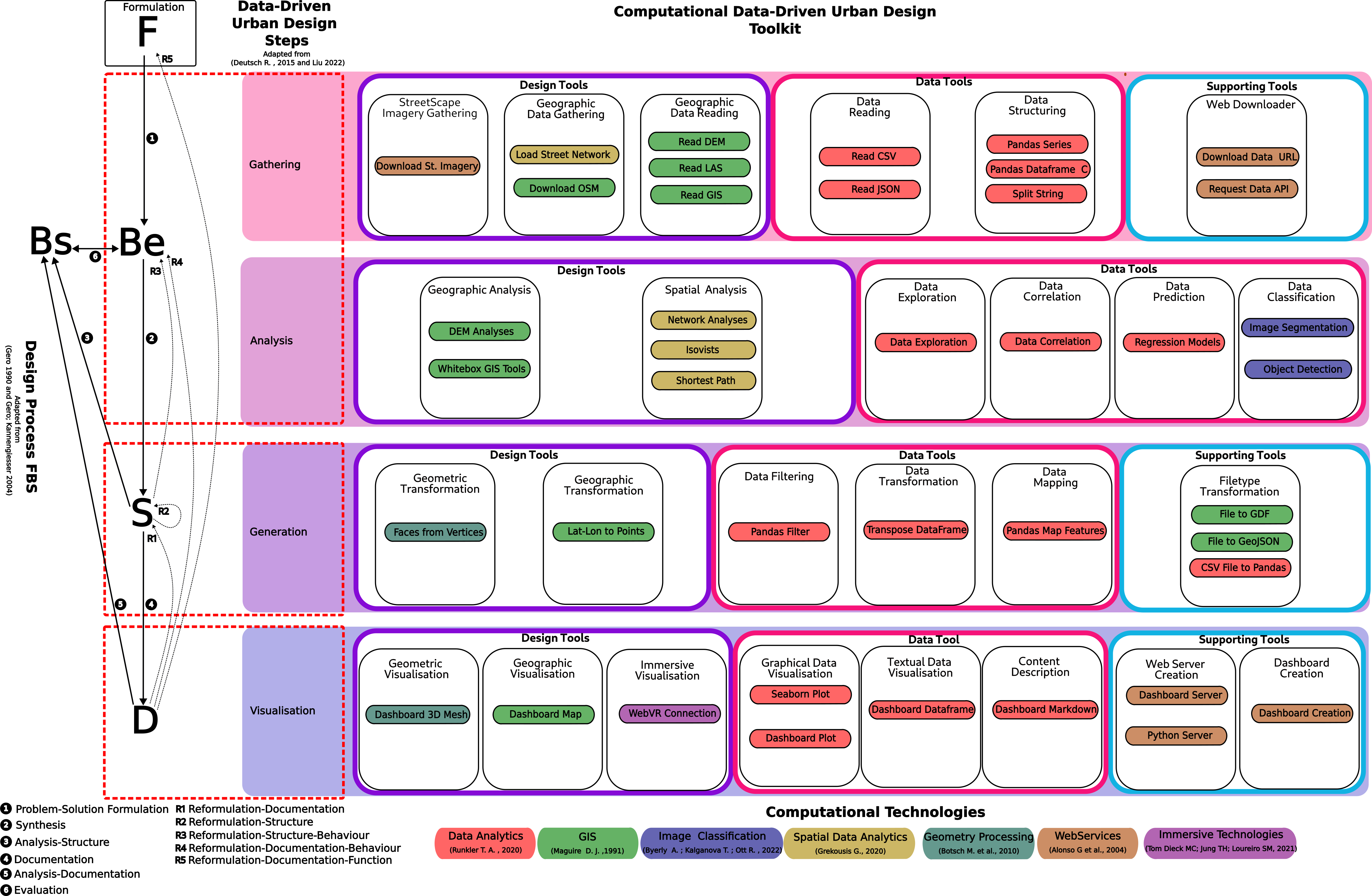
Figure 5.1: Mapping of Data-Driven Urban Design Processes Framework into Computational Toolkit
5.3 Computational Toolkit Prototype Development
The proposed computational toolkit prototype adopts a modular approach, categorising and dividing the tools according to the data-driven urban design steps: Gathering, Analysis, Generation, and Visualisation.
The next sections provide a detailed description of the implemented subcategories of data, design, and supporting tools in each step of the data-driven urban design process.
5.3.1 Gathering
This subsection describes the design, data, and supporting subcategories for the Gathering tools. As discussed in Chapter 4, it is during the data gathering phase that designers identify the data that will support the previous problem-solution formulation step in an iterative manner, with the functional requirements informing which type of raw data should be gathered and the exploration of the gathered data informing whether additional raw data should be gathered.
5.3.1.1 Design Tools
The Gathering Design Tools category is divided into three subcategories: Streetscape Imagery Gathering, Geographic Data Gathering, and Geographic Data Reading. These three categories provide a comprehensive set of options for gathering and reading urban design data in an integrated manner, including street imagery, GIS vector data, Digital Elevation Models, Point Clouds, and Street Networks.
The Streetscape Imagery Gathering tool provides remote visual information about the urban environment without a physical site visit. Additionally, recent research in environmental psychology has used such data to analyse the subjective qualities of urban spaces, such as Imageability, Enclosure, Human Scale, Complexity, and Transparency, using geo-referenced images and computer vision (Ewing and Clemente 2013; W. Qiu et al. 2021, 2022; Aman et al. 2022). The integration of the tool within a design environment facilitates more informed decision-making during the design process, by allowing designers to access and classify images and videos using advanced image segmentation and data analytics algorithms. The use of visual programming enhances interoperability and reduces the need for coding expertise or external software packages.
This functionality is implemented using a python library, which downloads data from the crowdsourced street imagery provider Mapillary.
Figure 5.2: Street Imagery Gathering Tool
The Geographic Data Gathering subcategory utilises GIS public services to download geodata. This subcategory employs the OpenStreetMap service to download GIS vector data, which is a free and open-source service that provides high-quality worldwide geodata that is produced and reviewed through a crowdsourced initiative. The Geographic Data Gathering category has two components: the Download OpenStreetMap tool uses the python library, osmnx, to download geographic vector data based on address, point, bounding box, or coordinates (Boeing 2017); and the Load Street Network tool, which loads street network data into Sverchok, including the topological structure of nodes and edges, which are cleaned and optimised for network analysis.
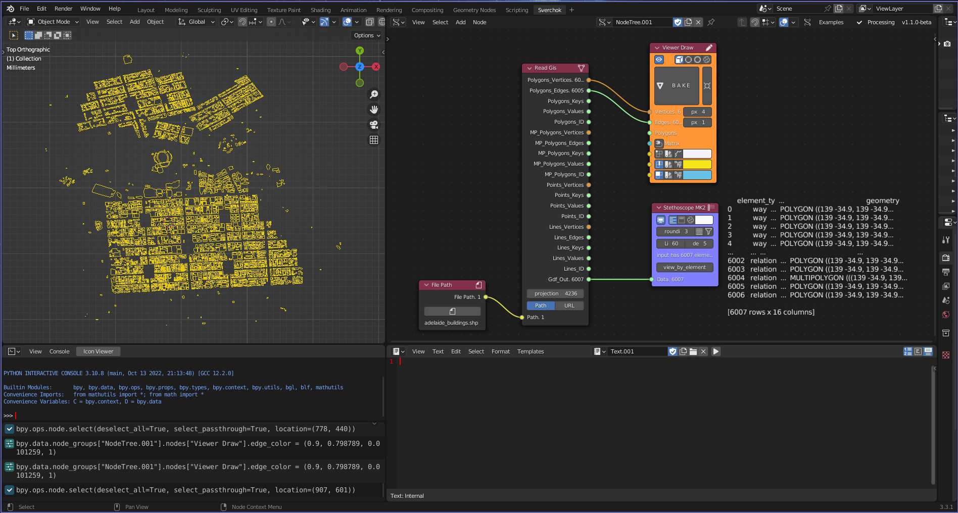
Figure 5.3: Read GIS Tool
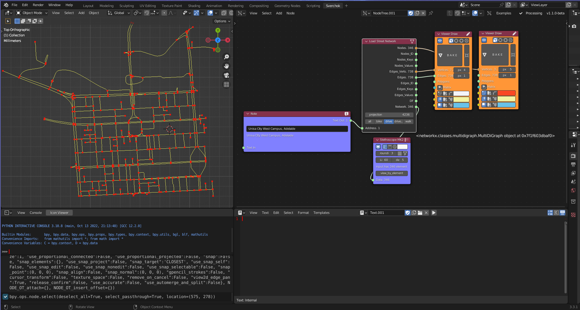
Figure 5.4: Load Street Network Tool
The Geographic Data Reading subcategory consists of three tools. The first tool, Read DEM, allows for the reading of Digital Elevation Models (DEM) to create high-fidelity topographic models using weighted raster files. This data type is widely used to understand geomorphological site formations, such as hydrological streams and topographic aspects, and plays a crucial role in landscape and urban design projects. The tool uses the python library rasterio to read elevation data from a GeoTIFF file and convert it into a Sverchok Mesh and a data frame with topographic values.
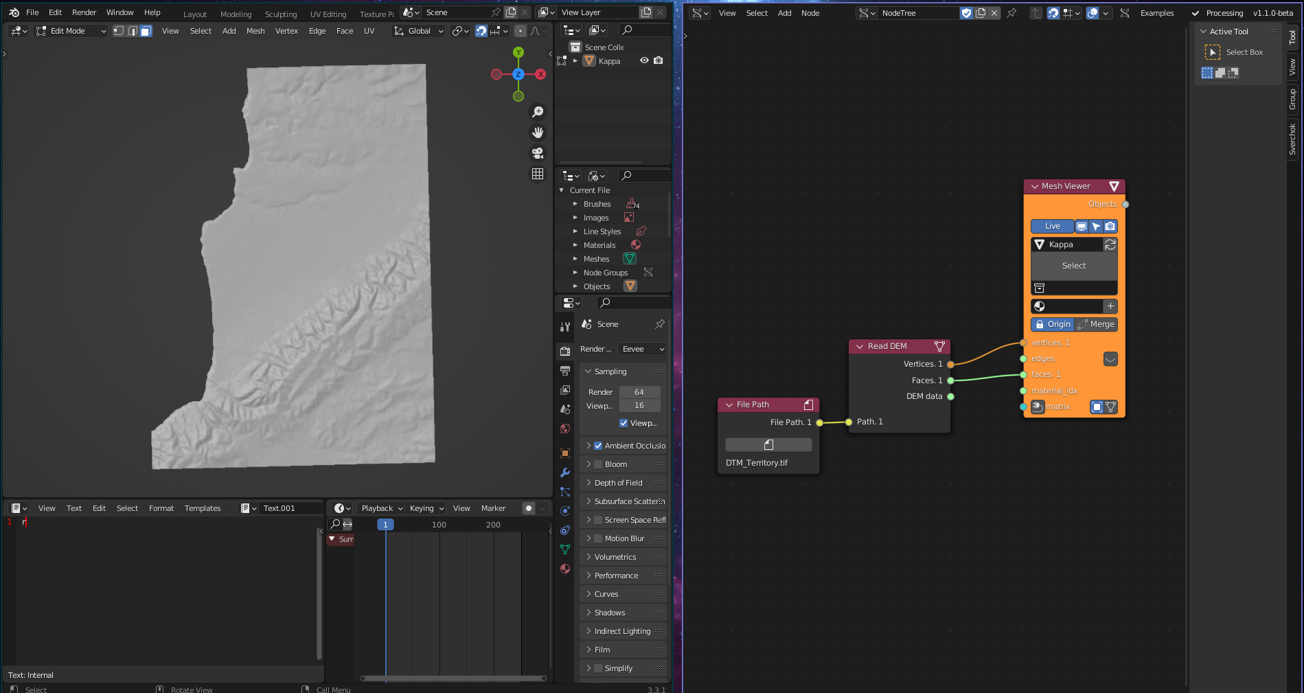
Figure 5.5: Read DEM Tool
The Read LAS tool is designed for reading point cloud LIDAR (Laser Imaging, Detection, and Ranging) data. LIDAR is a scanning mechanism that measures the variable distance to a surface or object by targeting it with a laser and measuring the time it takes for the reflected light to return to a receiver. Governmental portals around the world provide access to LIDAR datasets, which include built and natural urban environment features such as tree canopies and building heights. The tool for reading point cloud LIDAR data uses the python library laspy and converts the point cloud data into Sverchok vertices and a corresponding dataframe containing feature data (intensity and category) for each point.
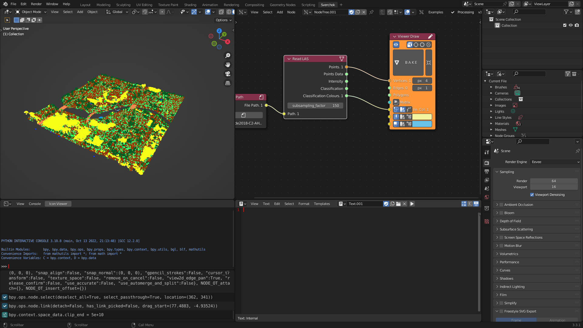
Figure 5.6: Read Las Tool
The Read GIS tool is a GIS vector reader that supports three file formats: geopackage, shapefile, and geojson. This tool is critical in providing structured geographic information about places, including geometries and properties related to each geometric element. The tool uses a python library, geopandas to read the GIS data, which is then converted into Sverchok meshes and associated feature data.

Figure 5.7: Read GIS Tool
5.3.1.2 Data Tools
The Gathering Data Tools category is divided into two subcategories: Data Reading and Data Structuring. These two categories provide tools for reading and structuring data in formats that are the industry standard for data analytics, integrating these data formats into a single design environment. Within the Data Reading subcategory, two tools have been developed: Read CSV and Read JSON.
Comma Separated Values (CSV) is a tabular data structure that is organised into rows and columns. This structure is widely used and supported across various fields and software packages (Nayak, Božić, and Longo 2022). The Read CSV tool utilises the standard python library to read CSV files, transforming the tabular data into a list, a dictionary, and a Dataframe within Sverchok.
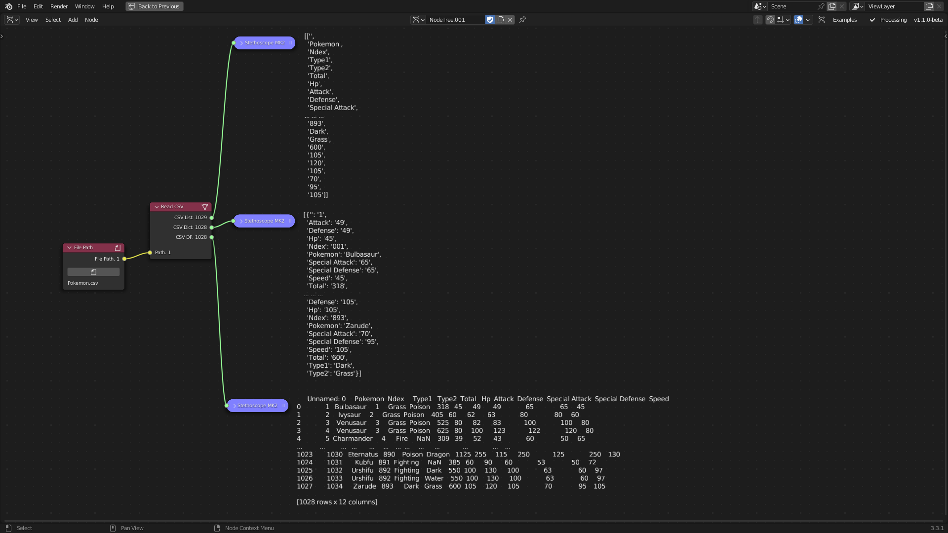
Figure 5.8: Read CSV Tool
The Read JSON tool is designed to integrate complex, nested data stored in JavaScript Object Notation (JSON) files into Sverchok. Unlike Comma Separated Values (CSV) files, JSON supports more intricate data structures, as it is composed of objects and attributes that can be nested and accessed based on a key-value pairing. The tool reads JSON files using the standard Python library, converting the file into a string of text and a DataFrame.
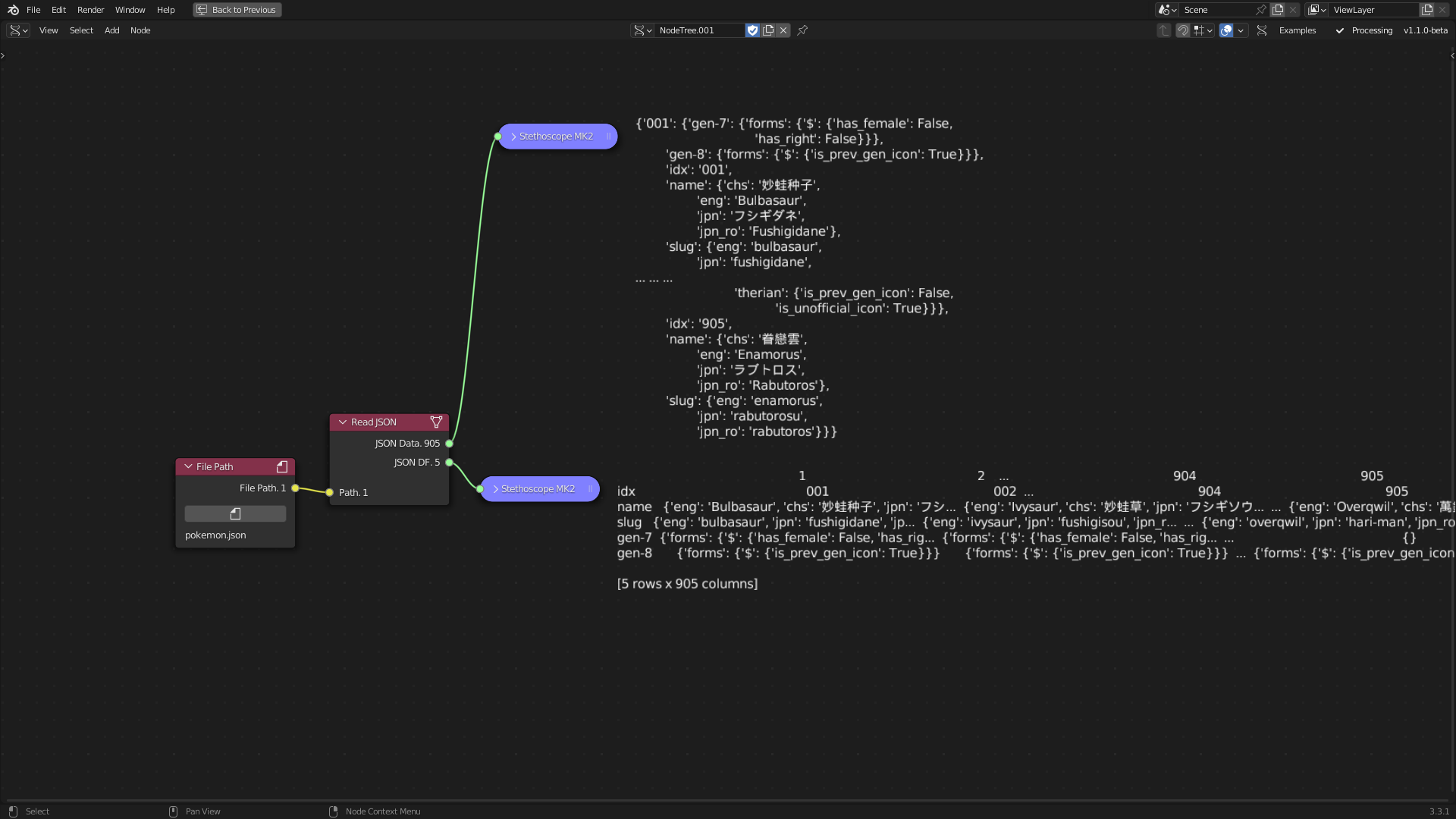
Figure 5.9: Read JSON Tool
The Data Structuring subcategory comprises three tools: Pandas Series, Pandas DataFrame Creation, and Split String.
The pandas library is a widely used data analysis tool for exploring, cleaning, and processing data (McKinney et al. 2011). The Pandas Series tool transforms Sverchok lists into Pandas Series, which are column-based data structures. Pandas Series can be combined to form a DataFrame, which is an indexed tabular structure. The Pandas DataFrame Creation tool is utilised to construct a DataFrame. The Split String tool employs standard Python functions to split text into a list of words, a feature that aids in cleaning and organising data.
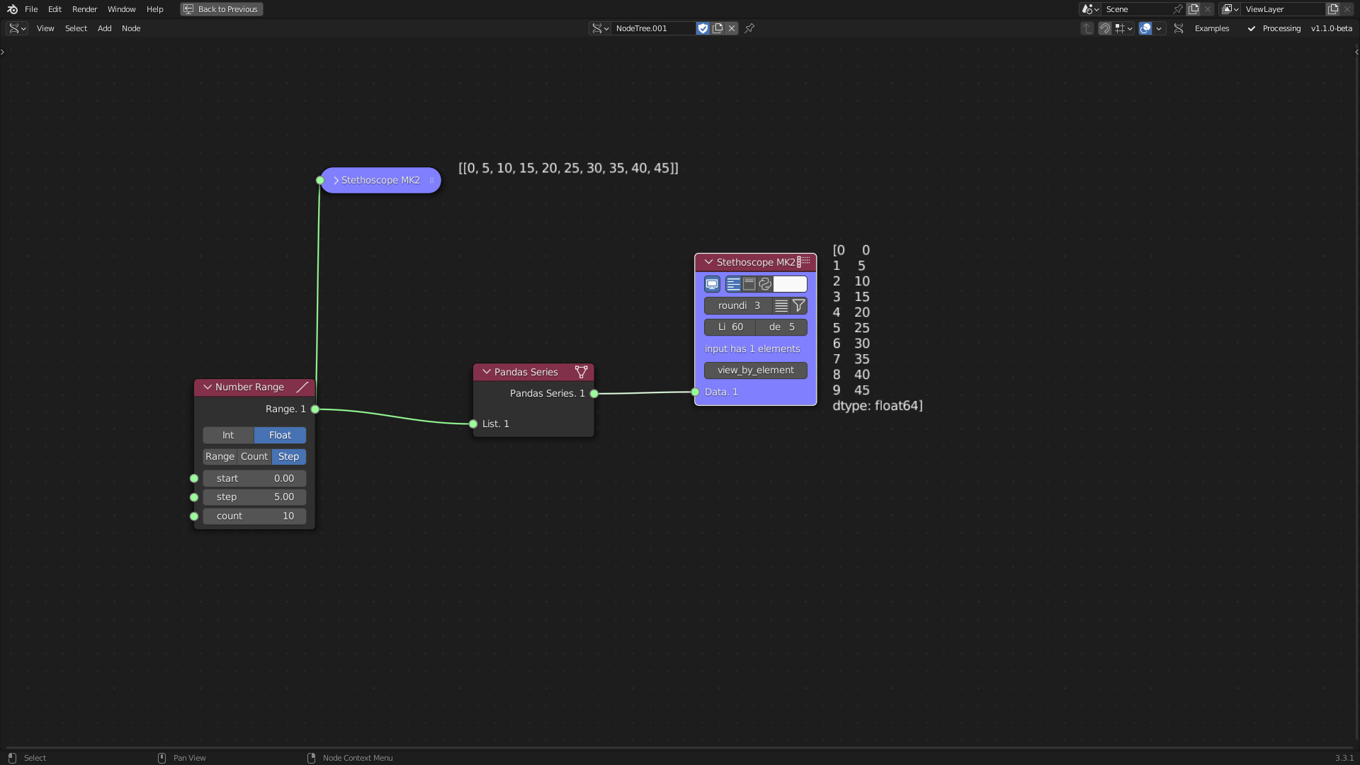
Figure 5.10: Pandas Series Tool
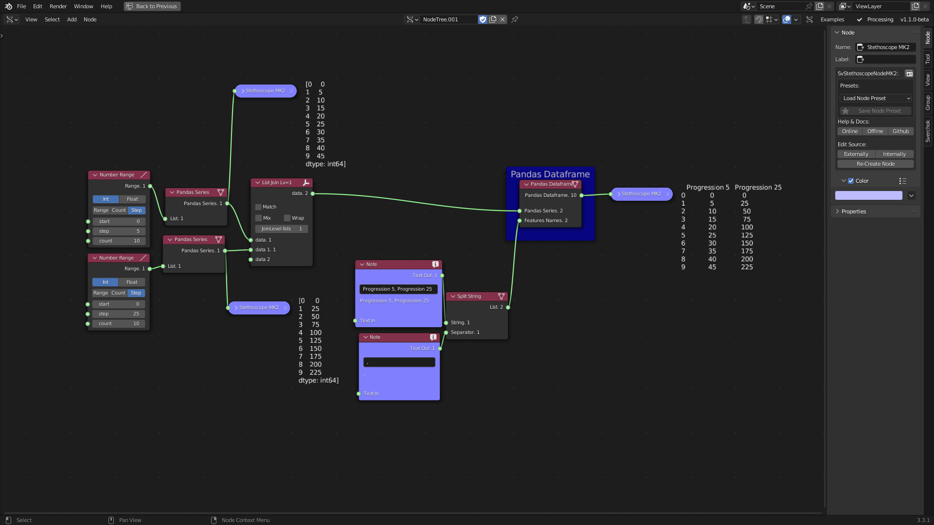
Figure 5.11: Pandas Dataframe Tool
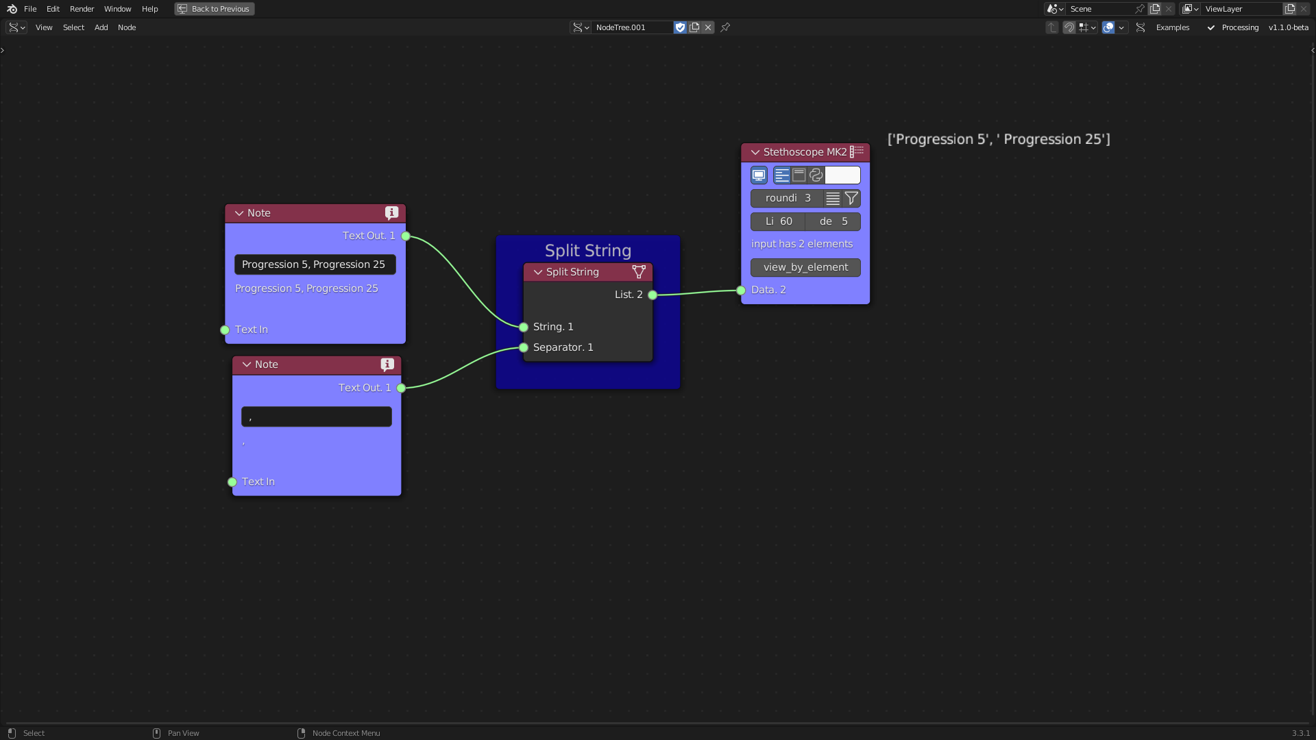
Figure 5.12: Split String Tool
5.3.1.3 Supporting Tools
The Gathering Support Tools category has a single subcategory, Web Downloader, which contains two tools: Download Data URL and Request Data API. This subcategory provides support in downloading and integrating data from public and available sources from the internet directly from the visual nodes.
The Download Data URL tool is a generic data downloader that uses the wget Python library. It downloads data from the internet using its URL.
Figure 5.13: Download Data URL
The Request Data API tool is used to download data from an Application Program Interface (API). The API provides the ability to filter, query, and manipulate data before downloading it. For instance, the Melbourne Pedestrian Count System uses an API to provide data access, which has compiled pedestrian data from Melbourne’s central business district since 2009. Utilising the API, the pedestrian data can be filtered and queried to specific periods before download. This tool is implemented using python library requests.
Figure 5.14: Request Data API Tool
5.3.2 Analysis
This subsection describes the design and data subcategories for analysis tools. The analysis step is a key part of the iterative problem-formulation process, as it, in combination with the data-gathering step, shapes the information that will inform the design requirements and goals, as well as whether further raw data needs to be collected. This process also provides inputs for the function (F) in the definition of specific objectives and informs the expected behaviour (Be) of the structure (S).
5.3.2.1 Design Tools
The Analysis Design Tools are divided into two subcategories: Geographic Analysis and Spatial Analysis. These two subcategories provide a comprehensive set of tools for realising geographic and spatial analyses in an urban design context, referring to Geographic Information Systems (GIS) and Spatial Data Analytics technologies, respectively. Despite similarities between these two categories, this research adopts separate subcategories due to the difference in the type of data they rely on. Geographic data relies solely on geo-referenced data, while the spatial data category can be used to manage both geo-referenced and non-geo-referenced data, such as mathematical relationships between geometry and topology.
The Geographic Analysis subcategory includes two tools: DEM Analyses and WhiteBox GIS Tools.
The DEM Terrain Attributes tool provides analysis for Digital Elevation Models (DEMs). When combined with the output of the Read DEM tool, the DEM Terrain Attributes tool returns values related to the geomorphological characteristics of the terrain, such as slopes, aspect, profile curvature, planform curvature, and standard curvature.
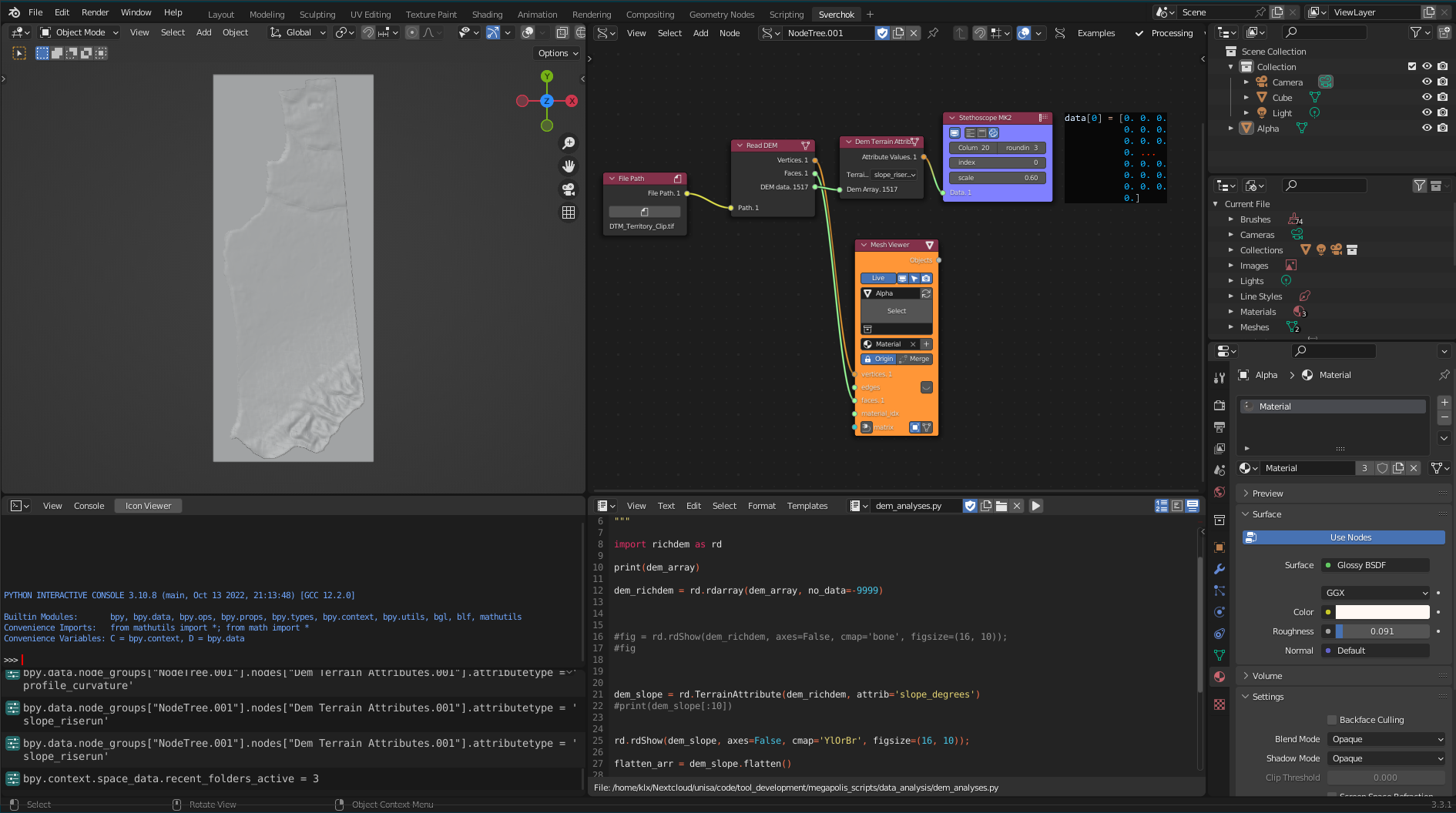
Figure 5.15: DEM Terrain Attributes Tool
The slopes are estimated based on a focal cell, calculating the centre difference of a surface fitted to the focal cell in relation to its neighbours. The slopes are defined as described in (Horn 1981):
The west-to-east slopes:
\[p_{w}=\frac{[(z_{++}+2z_{+0}+z_{-+}) - (z_{-+}+2z_{-0}+z_{--})]}{8\Delta y}\]
and south-to-north slopes:
\[q_{w}=\frac{[(z_{++}+2z_{0+}+z_{-+}) - (z_{+-}+2z_{-0-}+z_{--})]}{8\Delta y}\]
where slopes \(p\) (west-to-east direction) and \(q\) (south-to-north direction) are estimated from an array of elevations \(z_{00}\), which comprises elevations of adjacent grid points to the west and east, \(z_{-0}\), and \(z_{z+0}\), respectively. The adjacent grid points to the south \(z_{0-}\) and north \(z_{0+}\), which are similarly estimated. Also, the grid interval in the west-to-east is \(\Delta x\) in the same unit as the terrain elevations. The surfaces are estimated using a weighted average of the three central differences.
The aspect is estimated based on the direction of the maximum slope of the focal cell (Horn 1981). The steepest ascent using the same expression for the slope is defined by:
\[tan \theta = \sqrt{p^{2}+q^{2}}\]
where \(\theta\) is the angle of inclination of the surface.
The terrain curvature is estimated from the second derivate of the input surface value on the grid of points. For each cell, the surface \(Z\) is produced by the partial quartic equation (Zevenbergen and Thorne 1987):
\[Z = Ax^2y^2 + Bx^2y + Cxy^2 + Dx^2 + Ey^2 + Fxy + Gx + Hy + I\]
The relationships between the nine submatrix and nine elevation values are:
\(A = [(Z_{1} + Z_{3} + Z_{7} + Z_{9}) / 4 - (Z_{2} + Z_{4} + Z_{6} + Z_{8}) / 2 + Z_{5}] / L^4\)
\(B = [(Z_{1} + Z_{3} - Z_{7} - Z_{9}) /4 - (Z_{2} - Z_{8}) /2] / L^3\)
\(C = [(-Z_{1} + Z_{3} - Z_{7} + Z_{9}) /4 + (Z_{4} - Z_{6})] /2] / L^3\)
\(D = [(Z_{4} + Z_{6}) /2 - Z_{5}] / L^2\)
\(E = [(Z_{2} + Z_{8}) /2 - Z_{5}] / L^2\)
\(F = (-Z_{1} + Z_{3} + Z_{7} - Z_{9}) / 4L^2\)
\(G = (-Z_{4} + Z_{6}) / 2L\)
\(H = (Z_{2} - Z_{8}) / 2L\)
\(I = Z_{5}\)
where \(Z_{1}\) to \(Z_{9}\) are the nine submatrix elevations, \(Z_{5}\) is the centre point, and \(L\) is the distance (the same unit as \(Z\)) between grid points in both in the row and the column directions. Figure 5.16 presents a diagram 15 of this:.
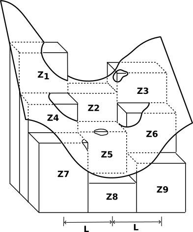
Figure 5.16: The relation between submatrix elevations, distances and the fitted surface, adapted from ArcGIS Repository Center
To calculate the curvatures (profile, planform, and standard), first the slope is derivate from \(Z\) regarding \(S\), where \(S\) is the aspect direction \(\theta\).
\[SLOPE= \partial Z/\partial S = Gcos\theta +H sin\theta\]
The \(cos\) and \(sin\) at the origin are, respectively (Zevenbergen and Thorne 1987):
\[cos\theta =-\frac{-G}{(G^2+H^2)^{1/2}}\]
\[sin\theta =-\frac{-H}{(G^2+H^2)^{1/2}}\]
Therefore, the slope is:
\[SLOPE= -(G^2+H^2)^{1/2}\]
The maximum slope direction (aspect) is defined as (Zevenbergen and Thorne 1987):
\[\theta = arctan (\frac{-H}{-G})\]
The signs of the numerator and denominator define the quadrant for \(\theta\), and the curvature \(\phi\) derivates from \(Z\) regarding \(S\) as (Zevenbergen and Thorne 1987):
\[Curvature =\frac{\partial Z^2}{\partial S^2} = 2(D cos^2 \phi + E sin^2 \phi +F cos \phi sin \phi)\]
From these equations, the profile curvature \(P_{c}\), planform curvature \(PL_{c}\), and standard curvature \(ST_{c}\) can be estimated.
The Profile Curvature runs parallels to the maximum slope of the surface, affecting the acceleration and deceleration of flows that go down the slope, as Figure 5.17 shows. The profile curvature is estimated based on a fitted surface to a local cell and its neighbours, and is defined as (Zevenbergen and Thorne 1987):
\[P_{c}= \frac{-2(DG^2+EH^2+FGH)}{G^2+H^2}\]
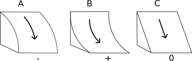
Figure 5.17: Profile Curvature based on ArcGIS Repository Center
The Planform Curvature runs perpendicularly to the maximum slope of the surface, affecting the convergence and divergence of flows that go down the slope, as Figure 5.18 shows. The profile curvature is estimated based on a fitted surface to a local cell and its neighbours, and is defined as (Zevenbergen and Thorne 1987):
\[PL_{c}= \frac{2(DH^2+EG^2-FGH)}{G^2+H^2}\]
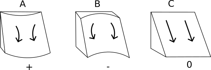
Figure 5.18: Planform Curvature
The Standard Curvature combines the Planform Curvature and the Profile Curvature, considering acceleration and deceleration as well as convergence and divergence of flows down the slope. The standard curvature is defined as (Zevenbergen and Thorne 1987):
\[K = \frac{(\partial^2 Z/\partial S^2)}{(1+(\partial Z/\partial S)^2)^\frac{3}{2}}\]
Figure 5.19: Standard Curvature
The second tool WhiteBox GIS tools integrates the WhiteBox Tool in Sverchok. The WhiteBox Tool is an advanced geospatial data analysis tool that contains more than 480 tools for processing various types of geospatial data (Lindsay 2016). This integration allows users to access WhiteBox Tools directly from Sverchok without the need to run an external program or write code.
Figure 5.20: Whitebox GIS Tool
The Spatial Analysis subcategory has three tools: Isovists, Network Analyses, and Shortest Path.
The Isovists is a set of visible points in an environment in relation to a single point of view (Benedikt 1979).
The Isovists can be either two-dimensional or three dimensional. The implemented function for calculating Isovists in the toolkit is two-dimensional. The two-dimensional isovists is defined as a set of line segments \(V_{x}\) from a point \(x\) to points \(v'\) on a boundary surface \(\partial V_{x} - R_{x}\), as defined by Benedikt (1979):
\[V_{x} = ([x,y']: v' \epsilon (\partial V_{x} - R_{x}))\]
and the length of the radials line segments:
\[l_{x, \theta}= d(x,v') = \left\| v'-x\right\| = [(v'{_{1}}^{2} - x_{2}^{1})]+(v'{_{1}}^{2}-x_{2}^{2})]^\frac{1}{2}\]
Figure 5.21 shows a two-dimensional isovists and a boundary surface composed of the connection of the end of line segments. In Urban Design, the isovists’ measurable geometric properties, such as area, number of connected edges, and perimeter length can help users to understand a visual perception of the environment (Carmona 2002).
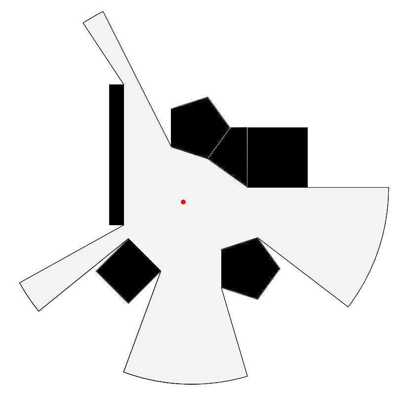
Figure 5.21: Isovist plane
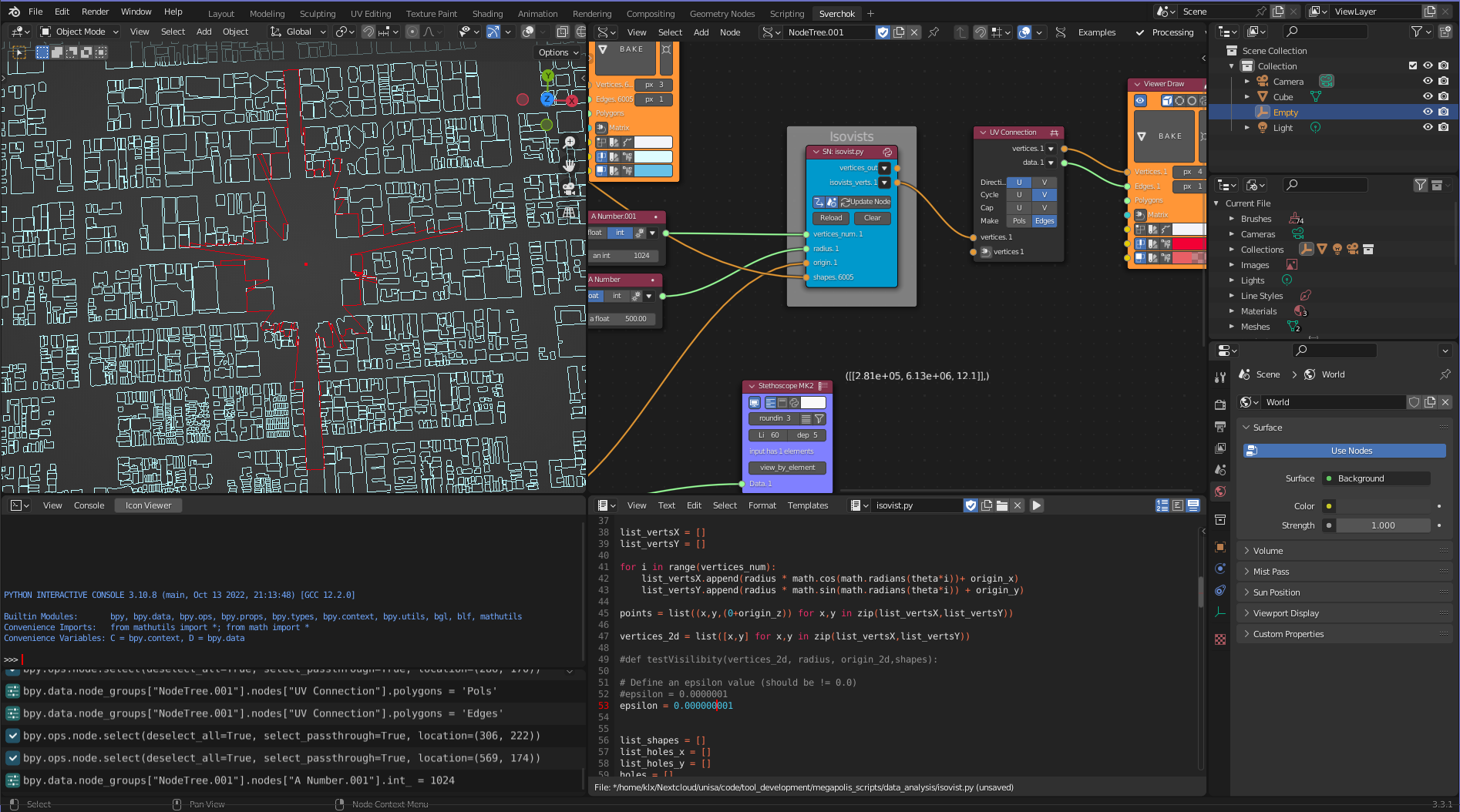
Figure 5.22: Isovist Tool
The Network Analysis tool is based on graph theory (Barnes and Harary 1983). A graph is a representation consisting of elements (nodes) connected to each other by edges (Trudeau 2013). In the context of an urban environment, nodes and edges represent the connections and intersections between streets, forming a street network (Barthélemy and Flammini 2008). Urban researchers have studied street networks to address various subjects, including transportation (W. E. Marshall and Garrick 2010) and urban form (Batty 2013b).
As a starting point for street network analysis, the Network Analysis tool implements three methods for measuring network centrality, as the centrality values can indicate accessibility (Batty 2013b): degree centrality, closeness centrality, and betweenness centrality.
Figure 5.23: Network Analysis Tool
The degree centrality measures how many connections a specific node has in the network. The degree centrality is defined as (Batty 2013b):
\[d_{j}=\sum_{i}g_{ij}\]
where the graph \(G(N,g)\) has a number of nodes \(N\) and \(g_{ij}\) is a link between a node \(i\) to a node \(j\).
The closeness centrality measures the average shortest path distance of a node of the network in relation to all other reachable nodes. The closeness centrality is defined as (Freeman 1977):
\[C_{i}=\frac{n-1}{\sum_{n-1}^{j=1}d(j,i)}\]
where the closeness centrality \(C\) from a node \(i\) in relation to a node \(j\) is the shortest path \(d(j,i)\), in which \(n-1\) is the number of reachable nodes \(j\) from the node \(i\).
The betweenness centrality indicates a fraction of shortest paths that pass through the nodes. The betweenness centrality is defined as:
\[C_{B}(v)=\sum_{s,t \epsilon V}\frac{\sigma (s,t|v)}{\sigma(s,t)}\]
where the betweenness centrality \(C_{B}\) of a node \(v\) is the sum of the fractions of all-pairs’ shortest paths that pass through \(v\), in which \(J\) is the set of nodes and \(\sigma(s,t)\) is the number of shortest \((s,t)\)-paths, and \(\sigma(s,t|v)\) is the number of those paths passing through some node \(j\) other than \(s,t\).
Shortest Path is a set of algorithms used to measure the shortest distance between nodes in a graph (Madkour et al. 2017). In an Urban Design context, the shortest path algorithms are used to study the connectivity of the urban environment (Batty et al. 1998; Kitazawa and Batty 2004).
A classic shortest path algorithm is Dijkstra’s algorithm (Dijkstra et al. 1959), which is defined in pseudocode as:
function Dijkstra(Graph, source):
for each vertex v in Graph.Vertices:
  dist[v] ← INFINITY
  prev[v] ← UNDEFINED
  add v to Q
dist[source] ← 0

while Q is not empty:
  u ← vertex in Q with min dist[u]
  remove u from Q

  for each neighbor v of u still in Q:
      alt ← dist[u] + Graph.Edges(u, v)
      if alt < dist[v]:
      dist[v] ← alt
      prev[v] ← u

return dist[], prev[]
where \(Q\) is used to store the unprocessed vertices with the estimated shortest-path. This algorithm can be used to solve any shortest-path problem involving a directed graph and non-negative weights (Huang, Lai, and Cheng 2009). The Shortest Path tool has two methods to calculate the shortest path between two nodes. The first is the shortest-path by distance, which calculates the shortest path based on the length of the edges. The second method uses time-travel as a weight to calculate the shortest path, which is implemented based on the streets’ maximum speeds.
Figure 5.24: Shortest Path Tool
5.3.2.2 Data Tools
The Analysis Data Tools category is divided into four subcategories: Data Exploration, Data Correlation, Data Prediction, and Data Classification. The first three subcategories pertain to Data Analytics, and are based on the steps used to create a model, while the fourth pertains to Image Classification technology. The four subcategories provide state-of-art machine learning methods to analyse urban data.
Exploratory Data Analysis (EDA) is a process of investigating data to uncover patterns and indications, guiding the direction of further analysis (Tukey et al. 1977). In the context of urban design, EDA aims to guide the formulation of design hypotheses and highlight the strengths and weaknesses of the analysed site. The Data Exploration subcategory contains one tool for EDA, Dataframe Utils.
The Dataframe Utils tool provides four basic methods for exploring the properties of a dataset: info, head, tail, and describe. The info method provides meta-information about the dataset, such as the object type, memory usage, number of columns, and number of null objects. The head and tail methods show the first (head) or last (tail) rows and columns, based on a predefined number. The describe method provides basic statistical information about the dataset, including the count of elements in each column, mean, standard deviation, minimum and maximum values, and data distribution (25%, 50%, and 75%).
Figure 5.25: Dataframe Utils Tool
The Data Correlation category is concerned with measuring the strength of association between two variables (Lindley 1990). A widely used method is the Pearson Correlation Coefficient (PCC), which is defined as (Benesty et al. 2009):
\[r=\frac{\sum(x_{i}-\bar{x})(y_{i} - \bar{y})}{\sqrt{\sum(x_{i}-\bar{x})^2\sum(y_{i}-\bar{y})^2}}\]
where \(r\) is the correlation coefficient, \(x_{i}\) the values of the x-variables, \(\bar{x}\) the mean values of the x-variables, \(y_{i}\) the values of the y-variables, and \(\bar{y}\) the mean values of y-variables. The Data Correlation subsection is composed of two tools: Correlation and Correlation With. Correlation computes a correlation matrix of a Dataframe. Correlation With computes a pairwise correlation between rows or columns in a Dataframe.
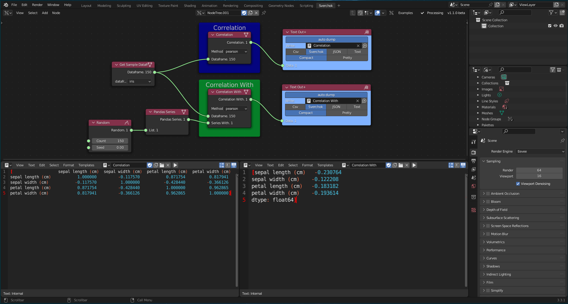
Figure 5.26: Correlation Tools
Data prediction involves a range of statistical techniques from data mining, predictive modelling, and machine learning. These techniques are used to infer future or unknown behaviours of datasets and establish relationships between variables (Fahrmeir et al. 2021). Regression models are a popular set of statistical techniques used in social sciences to make predictions. They estimate the relationship between a dependent variable and one or more independent variables. A linear regression model is a common type of regression model that estimates this relationship through a linear equation (Fahrmeir et al. 2021).
The Data Prediction subcategory in the Analysis Data Tools category includes four tools: Model Selection, Model Fit, Model Predict, and Model Evaluation. These tools support the creation of predictive models using linear regression algorithms such as Standard Linear Regression, RANSAC, Ridge, ElasticNet, and LASSO16. Linear models are fundamental for making predictions (Fahrmeir et al. 2021). The mathematical definition of the linear combination of features is provided by (Pedregosa et al. 2011):
\[\hat{y}(w,y)=w_{0}+w_{1}x_{1}+...+w_{p}x_{p}\]
where the vector \(w=(w_{1}...w_{p})\) contains the coefficients, \(w_{0}\) the intercept, and \(\hat{y}\) the predicted value.
The Data Classification subcategory comprises two tools: Object Detection and Image Classification.
Object detection algorithms detect instances of visual objects in an image or video based on a specific class of objects (Zou et al. 2019). Object detection has been widely used in various real-world applications, such as robot vision, surveillance, and autonomous vehicles (Zou et al. 2019). In the context of urban design, object detection has been explored in research to monitor urban activity and understand human behaviour in public spaces (Siewwuttanagul, Hayashida, and Inohae 2018; Massaro et al. 2021). The leading object detection algorithms currently are the R-CNN and YOLO series (Du 2018). Although the R-CNN has a higher accuracy in detection, it is slower compared with the YOLO series, making the latter more suitable for real-time detection applications (Du 2018).
The Object Detection tool utilises YOLO-v5 as the object detection framework. The tool can process detection of objects using inputs in the form of an image, webcam, camera IP, or video. The default detector can recognise 80 object classes, which are based on the Common Objects in Context (COCO) dataset (Lin et al. 2014). The results of object detection are saved in a CSV file as the tool’s output.
Figure 5.27: Object Detection
The Image Classification tool employs Detectron2 (Wu et al. 2019), which provides both object detection and image segmentation algorithms. Image Segmentation algorithms can categorise pixels with semantic labels (semantic segmentation), identify instances of objects (instance segmentation), or both methods combined (panoptic segmentation) (Minaee et al. 2022). Semantic segmentation involves labelling all individual pixels into object categories, such as trees, sky, and cars. Instance segmentation extends semantic segmentation by detecting and marking the instances of objects within an image.
The tool can receive an image, a folder of images, or a video as input, and perform instance and panoptic segmentation on the source. The image classification tool outputs the classified sources in a folder, as well as a CSV file that contains the classification results.
Figure 5.28: Image Segmentation
5.3.3 Generation
This subsection outlines the design, data, and supporting subcategories for generation tools. As discussed in Chapter 4, the generation process involves synthesis, analysis, and evaluation. The formulated design problem will inform the Expected Behaviour (Be) that is synthesised into a Structure (S), which is a potential solution. The Behaviour of the Structure (Bs) is then analysed against the Expected Behaviour (Be), as an Analysis of the Structure, to evaluate how the Behaviour of the Structure (Bs) performs. Designers and Data-Driven Designers negotiate between the problem and solution multiple times during the design process, while exploring design alternatives (Lawson 2006).
5.3.3.1 Design Tools
The Generation Design tool category within the proposed toolkit addresses the missing features of the standard Sverchok tools. It is divided into two subcategories: Geometric Transformation and Geographic Transformation. The former refers to Geometric Processing and the latter refers to GIS. These two subcategories provide simple generation tools that can be integrated with the existing Sverchok tools to complement features lacking in the generation of 3D urban models.
The Geometric Transformation subcategory contains a single tool, Faces from Vertices, which transforms vertices into faces. The tool implements a simple algorithm to achieve this.
Figure 5.29: Faces from Vertices
The Geographic Transformation subcategory has a tool called Latitude-Longitude to Points. This tool transforms a set of Latitude-Longitude pairs into (x, y) coordinates based on a specified Coordinate Reference System (CRS) projection.
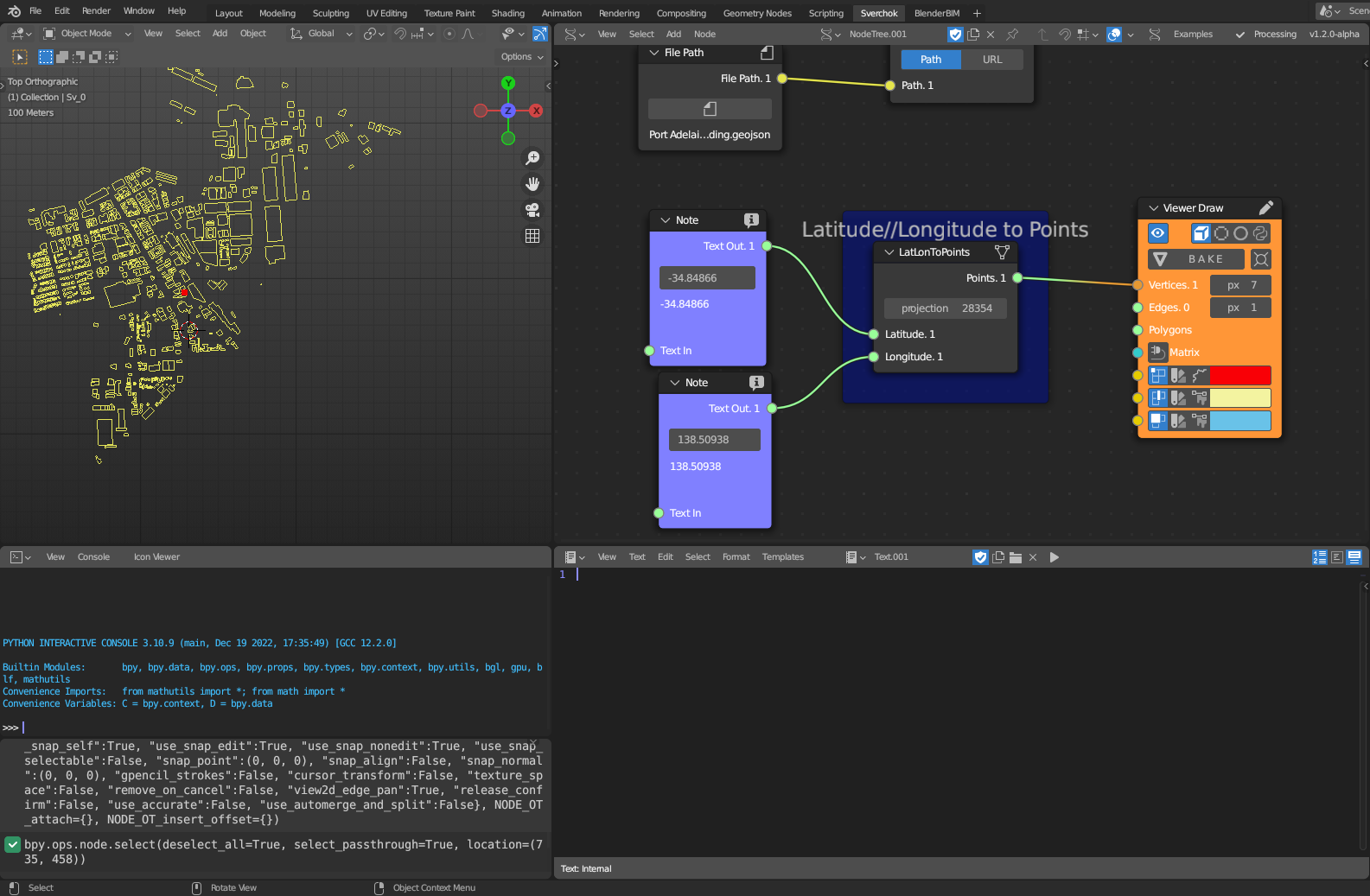
Figure 5.30: Latitude and Longitude to Points
5.3.3.2 Data Tools
The Generation Data Tools category is further divided into three subcategories: Data Filtering, Data Transformation, and Data Mapping. These subcategories fall under the umbrella of Data Analytics technology and are used to generated new data structures from existing ones.
The Data Filtering subcategory comprises one tool: Pandas Filter. This tool allows users to select a single feature column based on its feature name.
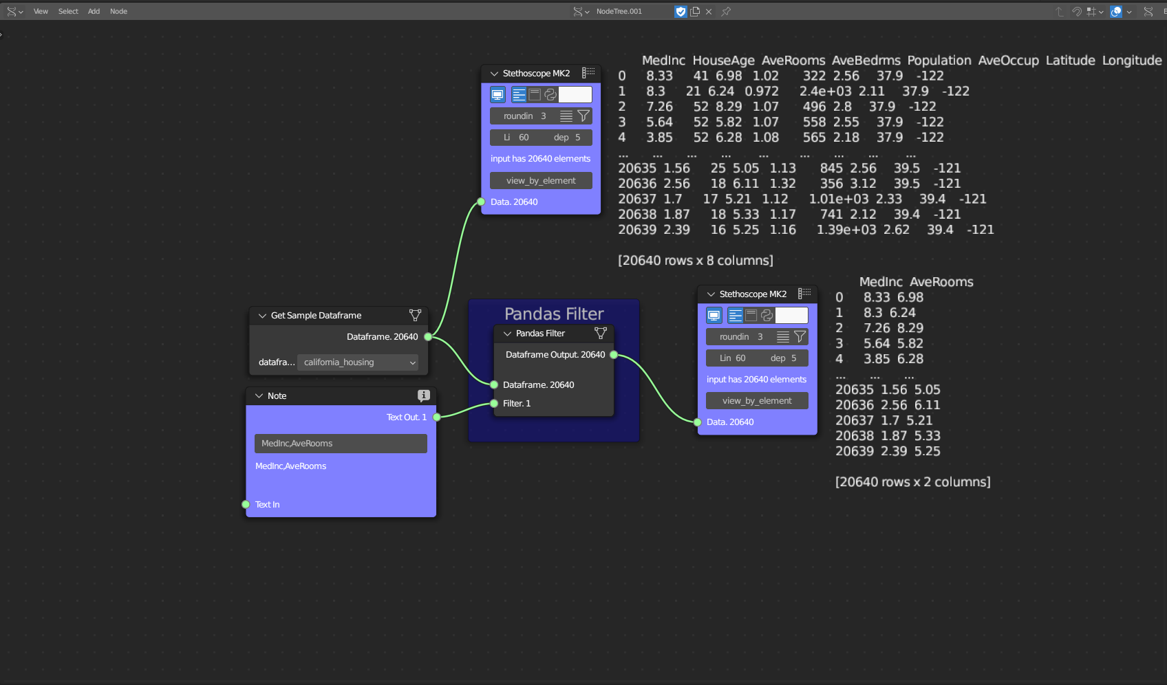
Figure 5.31: Pandas Filters
The Data Transformation subcategory has one tool: Transpose Dataframe. This tool transposes columns into rows.

Figure 5.32: Transpose Dataframe
The Data Mapping subcategory has one tool: Pandas Map Feature. This tool replaces each value from a feature with another value.
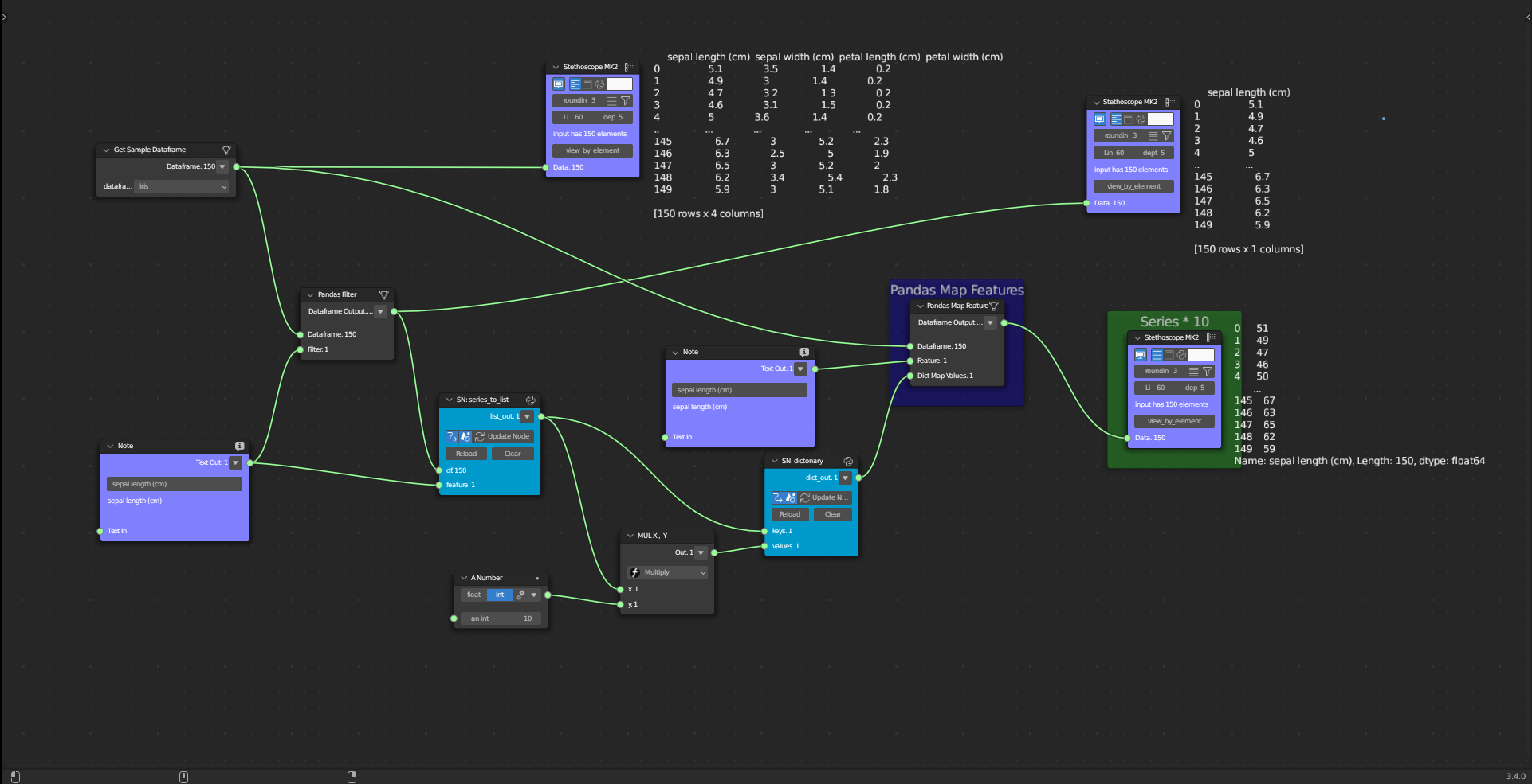
Figure 5.33: Pandas Map Features
5.3.3.3 Supporting Tools
The Generation Supporting Tools category encompasses one subcategory: File Type Transformation. This subcategory pertains to both GIS and Data Analytics technologies. This category supports transformations between different file types and data structures.
The File Type Transformation subcategory includes two tools: File to GDF and File to GeoJSON. These tools facilitate file transformations. The File to GDF tool takes in a shapefile, geopackage, or geojson file and loads its data as a GeoDataFrame. The File to GeoJSON tool, on the other hand, receives a shapefile or geopackage file and loads its data as GeoJSON.
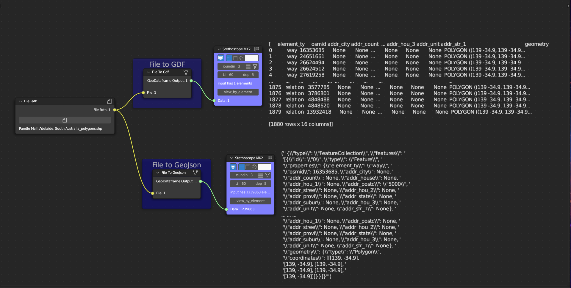
Figure 5.34: File to GDF and File to GeoJSON
5.3.4 Visualisation
This subsection outlines the design, data, and supporting subcategories for visualisation tools. The visualisation step is an interactive and iterative process of representing potential solutions, with the visual outcome informing the Behaviour Structure (Analysis-Documentation) through the analysis of the documentation. As discussed in Chapter 4, this is a key element of data-driven design since, in traditional design, the visualisation is usually a static representation of the final solution, whereas in data-driven design it can provide new insights into the exploration of the solution space of the design process.
5.3.4.1 Design Tools
The Visualisation Design Tools category is divided into three subcategories: Geometric Visualisation, Geographic Visualisation, and Immersive Visualisation. These three subcategories correspond to the Geometric Processing, GIS, and Immersive Technologies, respectively. These three subcategories provide a comprehensive and interactive set of tools for creating visualisations in an integrative manner.
One of the key features of the Visualisation Tools is the use of interactive dashboards. Dashboards have been widely utilised in industry to support data-driven decision-making (Sarikaya et al. 2018). In a data-driven urban design process, dashboards can provide an interactive, participatory space where different stakeholders can collaborate and share ideas without the need for knowledge of a visual programming tool. Thus, the implementation of interactive dashboards is a main strategy for visualisation, using python library streamlit.
The Geometric Visualisation subcategory includes one tool, Dashboard 3D Mesh, which creates an interactive 3D representation in a dashboard. This tool takes a 3D mesh as input.
Figure 5.35: Dashboard 3d Mesh
The Geographic Visualisation subcategory comprises a single tool, known as the Dashboard Map. This tool creates an interactive web map that is embedded within a dashboard. The input required for this tool is a Geodataframe.
Figure 5.36: Dashboard Map
The Immersive Visualisation subcategory includes a single tool, the WebVR Connection. This tool is an interactive WebVR webpage created using the A-Frame WebVR framework.
Figure 5.37: WebVR Connector
5.3.4.2 Data Tools
The Visualisation Data Tools category is divided into three subcategories: Graphical Data Visualisation, Textual Data Visualisation, and Content Description. These subcategories relate to the technology of Data Analytics and provide tools for visualising data through graphs and text, as well as creating descriptions to support urban design narratives.
The Graphical Data Visualisation subcategory encompasses two tools: the Seaborn Plot and the Dashboard Plot. The Seaborn Plot employs the seaborn library (Waskom 2021) to plot graphs from data frames. The Dashboard Plot generates an interactive plot within a dashboard.
Figure 5.38: Seaborn Plot (Pair Plot)
The Textual Data Visualisation subcategory includes a single tool, the Dashboard Dataframe. This tool plots the tabular content of a dataframe in an interactive dashboard.
Figure 5.39: Dashboard Dataframe
The Content Description subcategory includes a single tool, the Dashboard Markdown. This tool takes a Sverchok text block and displays its content within an interactive dashboard.
Figure 5.40: Dashboard Markdown
5.3.4.3 Supporting Tools
The Visualisation Supporting Tools category is divided into two subcategories: Web Server Creation and Dashboard Creation. These subcategories relate to the technology of Web Services. These supporting categories are used to create the background servers that will allow the visualisation of the data in an internet browser.
The Web Server Creation subcategory encompasses two tools. The first tool, the Dashboard Server, creates a web server to run the dashboard. The second tool creates a Python server that can be used to run the WebVR webpage.
The Dashboard Creation subcategory includes a single tool, Dashboard Creation. This tool compiles all dashboard functions to generate a single dashboard file.
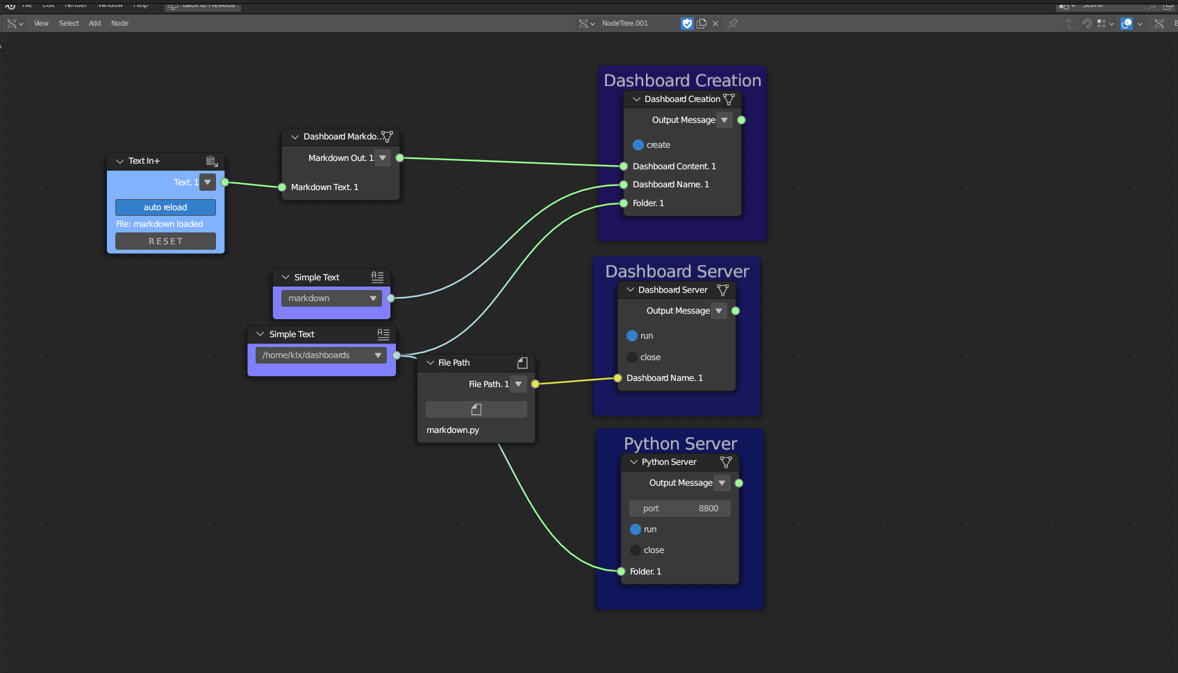
Figure 5.41: Visualisation Supporting Tools (Dashboard Server, Python Server, and Dashboard Creation)
5.4 An Urban Design Scenario for Demonstration
As described in Chapter 3, a demonstration was conducted using Port Adelaide as a scenario to showcase the implemented computational toolkit. The one-hour long demonstration was pre-recorded and uploaded to YouTube17. The nodes were presented in the context of Port Adelaide, highlighting the integration of data and design tools through the data-driven steps of Gathering, Analysis, and Visualisation. No design proposal was made during the demonstration, so the Generation step was not presented in the context. However, some Generation nodes were integrated during the other steps to support the workflow.
The focus of the demonstration was to present the nodes’ functionalities and their usability in a real-world scenario, rather than to perform a design exercise exploring alternative design options. As such, no design proposals or quantifications of analysis were made during the demonstration.
The scenario is divided into four parts, which are presented in the following subsections: Setup and Interface, Gathering, Analysis, and Visualisation.
5.4.1 Setup and Interface
As outlined in Chapter 3, the computational toolkit, called MEGA-POLIS18, is a plugin developed for Blender-Sverchok. In order to use this toolkit, it is necessary to first install Blender19 and Sverchok20.
Once Blender and Sverchok are installed, MEGA-POLIS can be downloaded from GitHub and installed. This toolkit supports GNU-Linux distributions such as Debian, Ubuntu, and Arch Linux, as well as Windows operating systems. Installation instructions can be found on the GitHub page.
After installation, the computational toolkit can be found within the Sverchok Menu by pressing Shift + a in the Sverchok viewport. The interface is organised following the framework structure presented in Section 5.2, and is divided into sub-menus for Gathering, Analysis, Generation, and Visualisation. Each sub-menu is further subdivided into tools categorised as Data, Design, or Supporting Tools. The interface is illustrated in Figure 5.42.
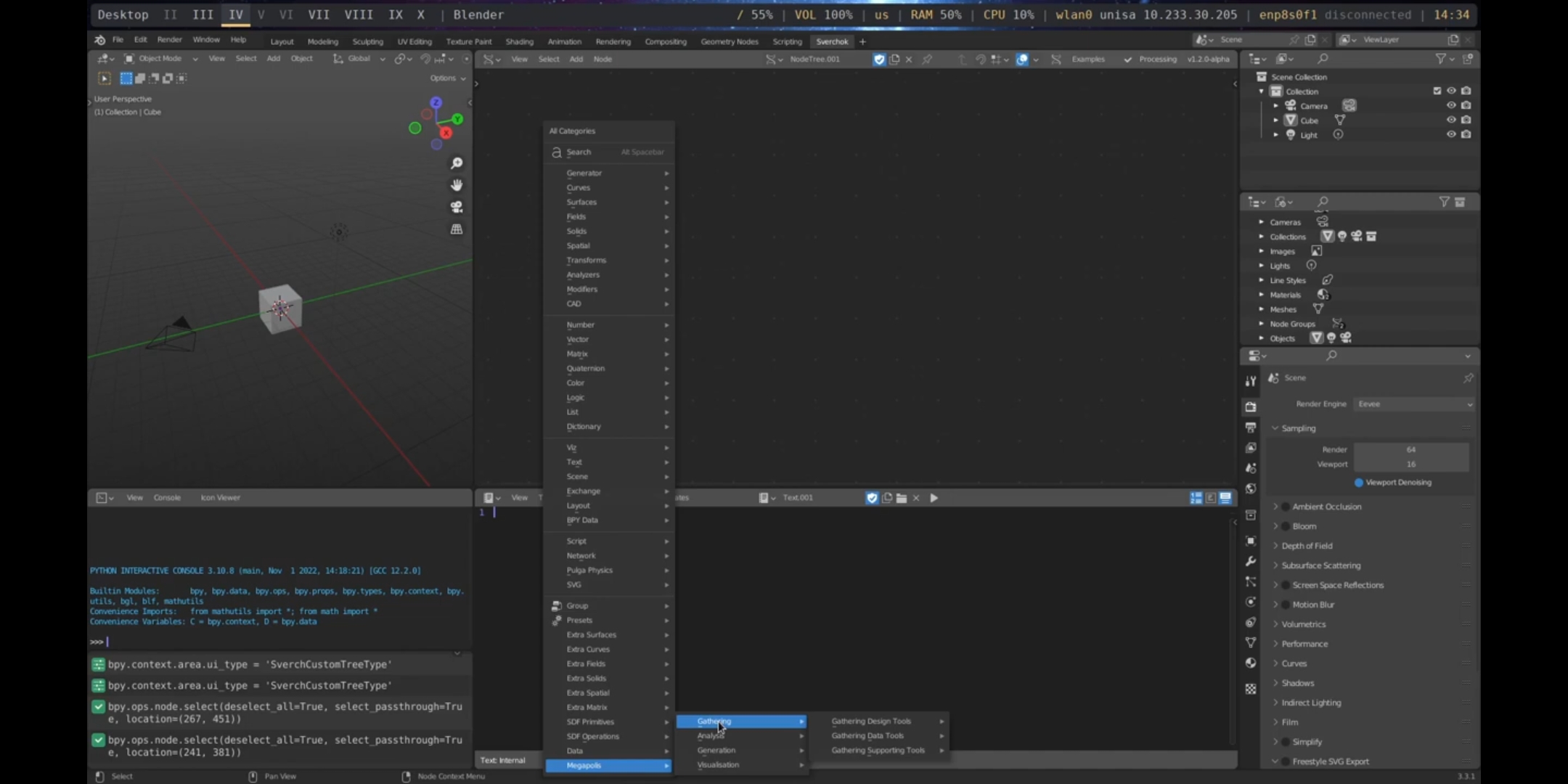
Figure 5.42: Computational Toolkit Interface
5.4.2 Gathering
In the Port Adelaide scenario, the first step explores the process of gathering data about the scenario. As discussed in Chapter 4, the gathering process is crucial to integrate required data used to build the design narrative. Generally, this data is gathered from different data sources and different pieces of software are required to manage those data. In the proposed implementation, different open-source services OpenStreetMap21 and Mapillary22) and support for different file formats (e.g., shapefile, geopackage, geoJSON, csv, JSON, geoTIFF, las, among others) are integrated into the visual programming environment facilitating the workflow.
Table 3.2 in Chapter 3 presents the data gathered for the Port Adelaide demonstration scenario. The gathering process is divided into two parts: gathering design and gathering data, following the structure outlined in the framework in Section 5.2.
5.4.2.1 Gathering Design
The first tool utilised is the Download OpenStreetMap, which is used to obtain the building footprints of the designated area. The parameters specified include the Address as Port Adelaide, City of Port Adelaide Enfield, South Australia, the feature being downloaded as building, which specifically retrieves building footprints, the Distance radius is set as 3000, and there is a specified Folder for the downloaded files. This configuration allows for the retrieval of all building footprints within a 3000-meter radius from the origin point specified by the address in Port Adelaide. The acquisition of building footprints is crucial in contextualising any urban design project.
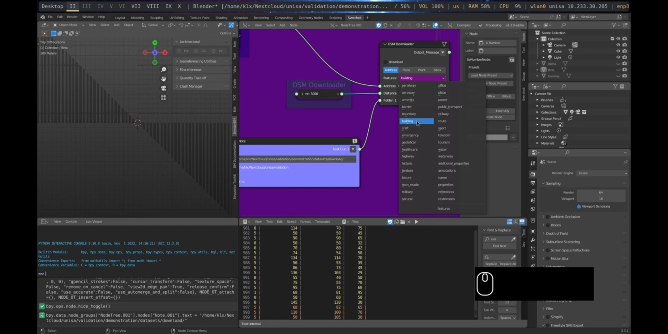
Figure 5.43: OSM Downloader Port Adelaide
The Read GIS node was utilised to load the downloaded GeoJSON file. Both the geometric and feature data were accessible as outputs from the Read GIS node. The correct projection parameter was set to 28354 to orient and correctly scale the geometries. It is crucial to ensure the proper setting of the Coordinate System Reference to the appropriate Universal Transverse Mercator (UTM) zone, as failure to do so may result in misalignment between other file formats such as digital elevation models and point clouds, thereby compromising the integration of various methods and file formats.
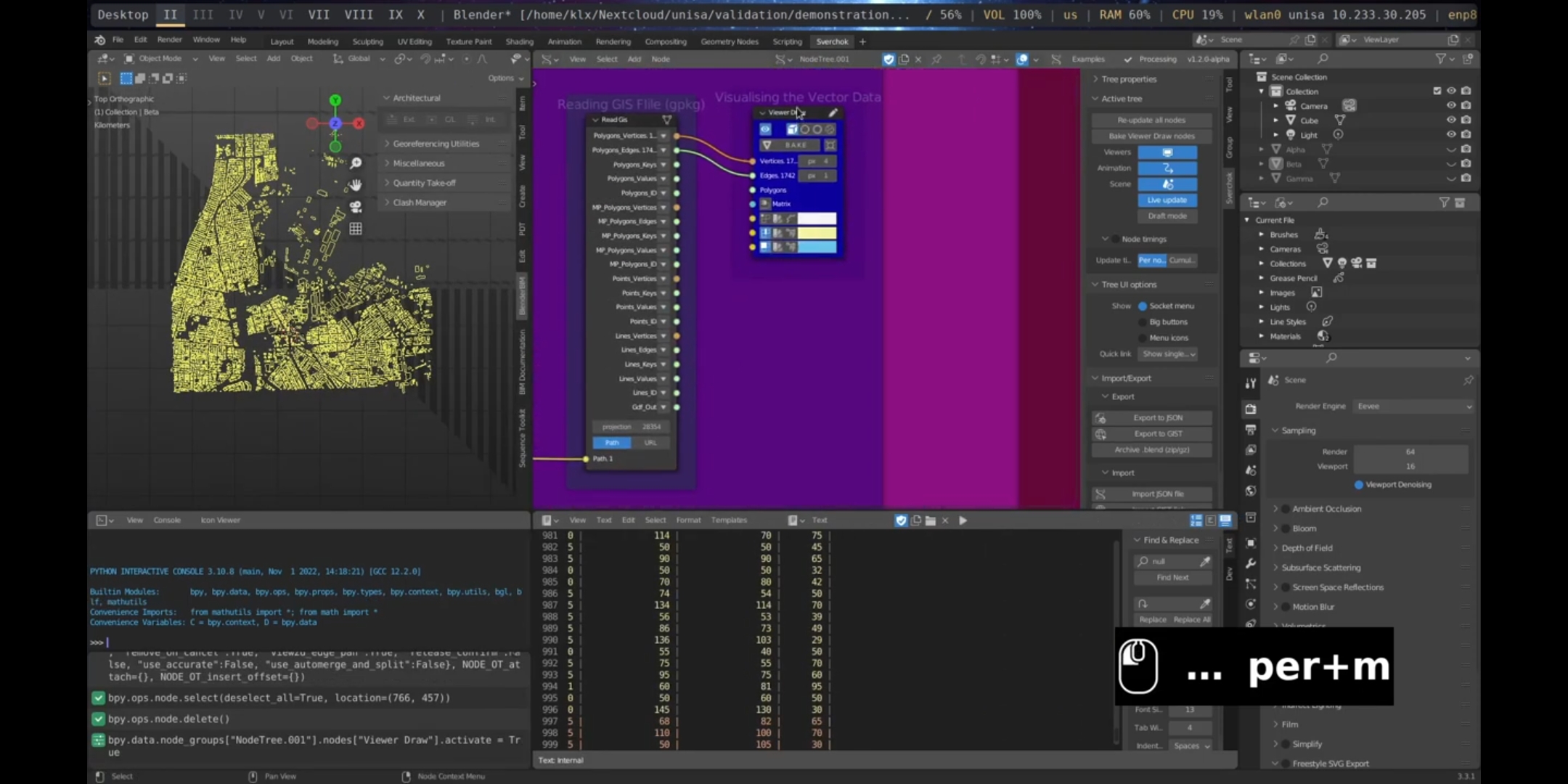
Figure 5.44: Read GIS Port Adelaide
Next, the street network was obtained using the same address and parameters utilised for retrieving the building footprints. The street network was downloaded ready optimised for conducting street network analysis, ensuring that there were no duplicated or overlapping lines. Furthermore, the model containing the street network’s structure (Nodes and Edges) was loaded, as this structure is fundamental for carrying out spatial analysis measurements.
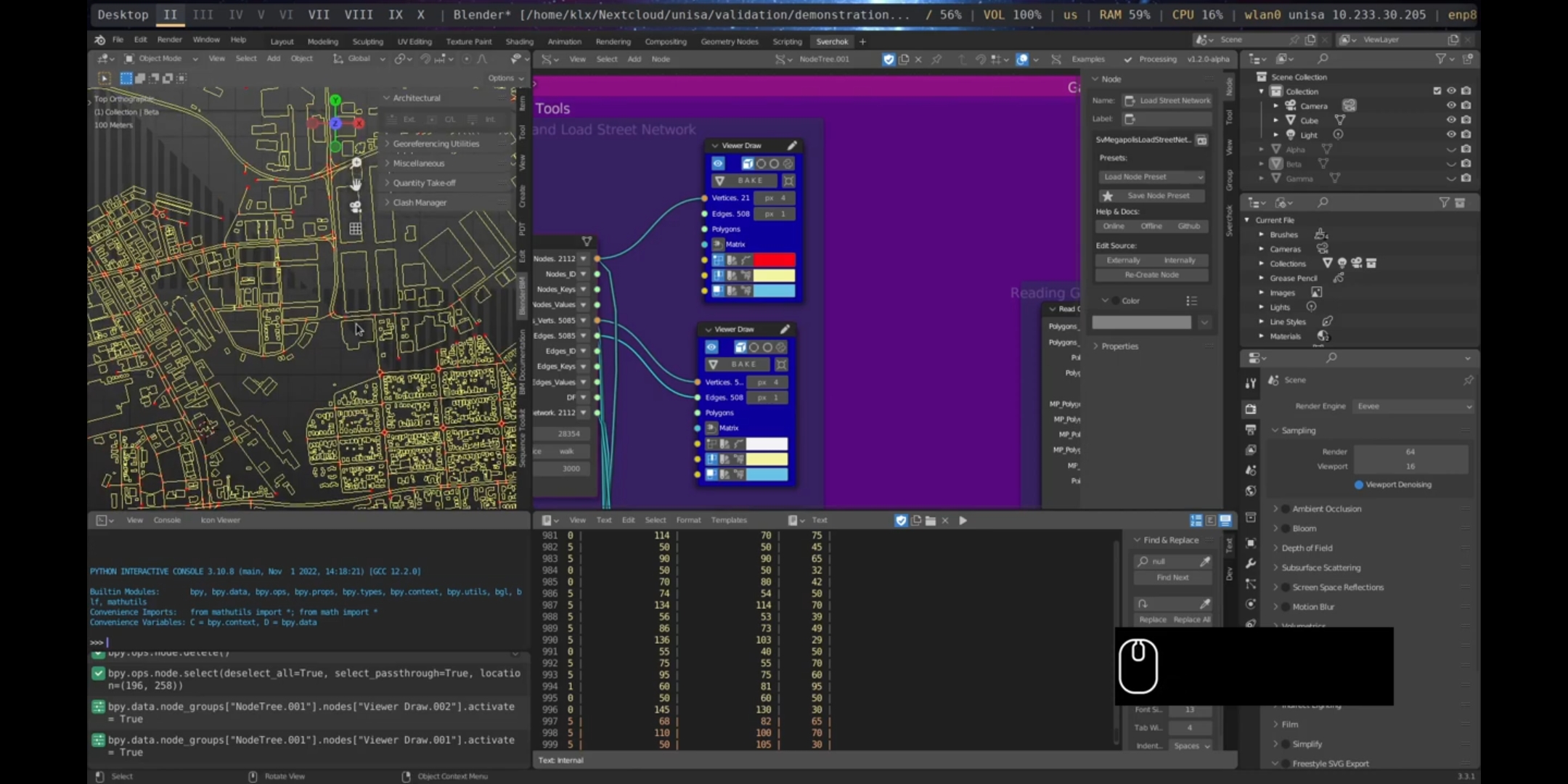
Figure 5.45: Street Network Port Adelaide
Data obtained from Elvis - Elevation and Depth - Foundation Spatial Data23 was utilised to load a point cloud model representing the 3D shape of a region in Port Adelaide from 2019. Additionally, a digital elevation model was downloaded from Elvis - Elevation and Depth - Foundation Spatial Data, providing the topographic information of the area.
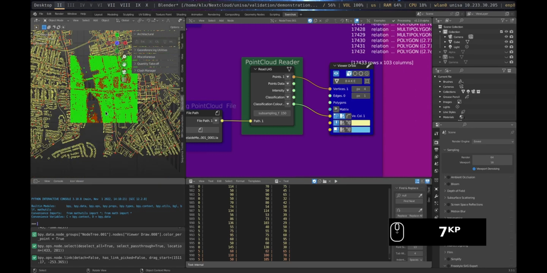
Figure 5.46: Point Cloud Port Adelaide
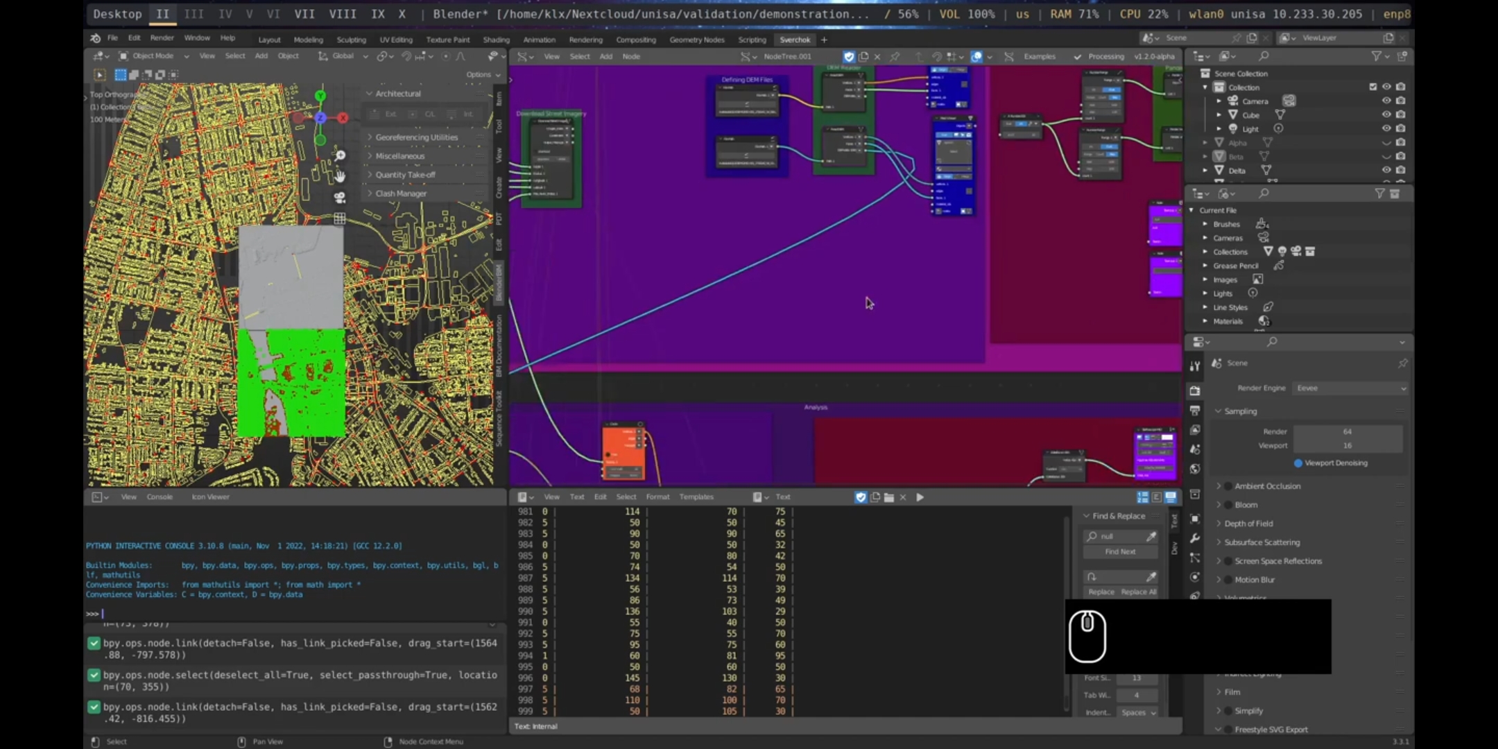
Figure 5.47: Digital Elevation Model, Port Adelaide
Finally, street imagery for the area was obtained from Mapillary using the Download Street Imagery Node. This imagery was utilised to assess the characteristics of the location. As shown by recent research (W. Qiu et al. 2021; Ye et al. 2019), online street imagery can be used to analyse the urban design qualities of a space through the implementation of advanced image segmentation algorithms. Therefore, this study employs an Image Segmentation node (refer to Subsection 5.4.3.2) that can be utilised in conjunction with the Download Street Imagery Node to facilitate this workflow.
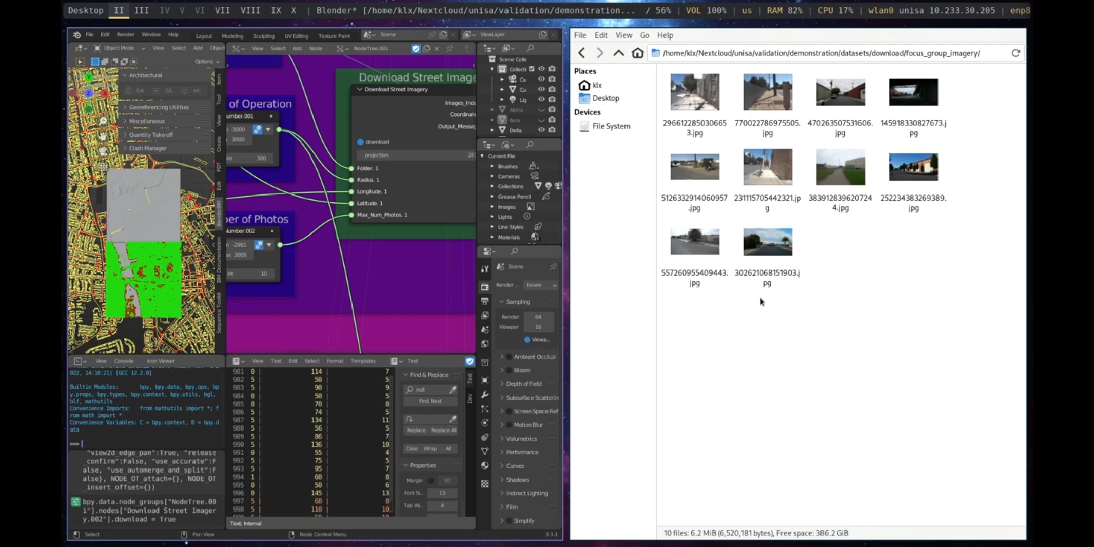
Figure 5.48: Download Street Imagery, Port Adelaide
One of the primary advantages of utilising the proposed environment to load diverse geospatial data is the capacity to integrate these diverse data types within a design framework.
5.4.2.2 Gathering Data
The first tool introduced in the “Gathering Data” section is the Request Data API node. This node enables the downloading of data from publicly available APIs by making a request. In the presented example, metadata from historical photos of Port Adelaide from 1840-1990, which are available on the DataSA24 portal through an API connection, were accessed using this node.
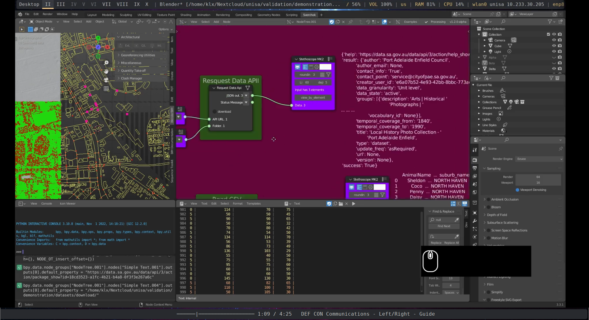
Figure 5.49: Request Data API Port Adelaide
Another important aspect in the data gathering process is the ability to read CSV files, as it is a widely distributed format across publicly available sources and essential for data analytics processes. In the demonstration, a dataset about animal registration in the Port Adelaide area (gathered from the DataSA portal) was loaded using the Read CSV node. This node provides outputs in different formats (Python List, Dictionary, and DataFrame), allowing for manipulation of the data in various ways.
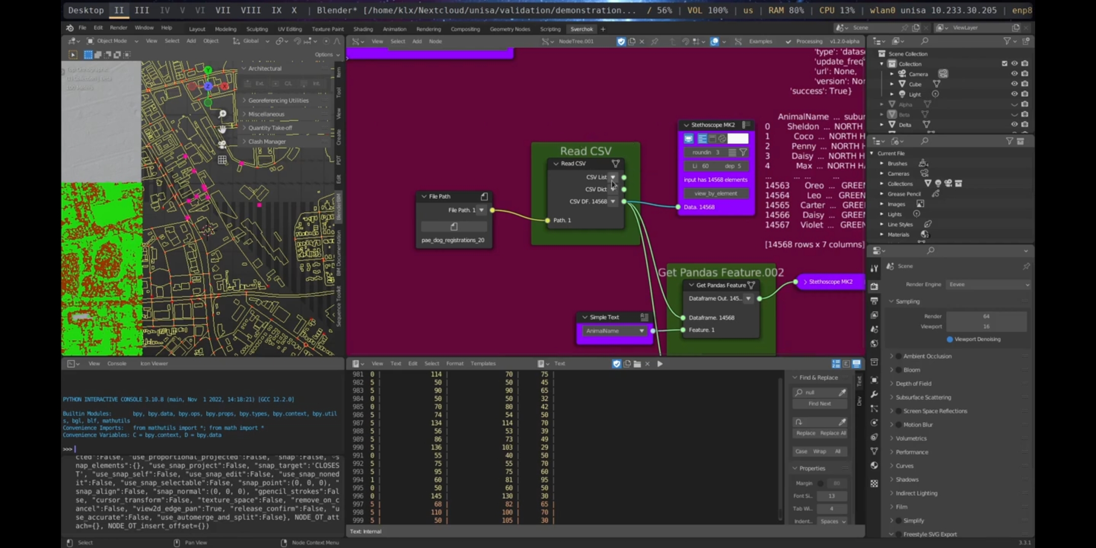
Figure 5.50: Read CSV Port Adelaide
The use of the Pandas25 dataframe structure is widely accepted in data analytics. It is a tabular format that provides a wide range of feature-rich operations, making the processing of data easier. In the demonstration, Sverchok lists are transformed into a dataframe structure using several nodes. Firstly, the Pandas Series node is utilised to create a dataframe feature column. Secondly, the Pandas Dataframe node is used to join columns into a tabular format. Finally, the Get Pandas Series node is used to select specific features from the dataframe, extracting one column from the dataframe as a pandas series. The interoperability between these different data structures is crucial for seamless integration of design and data.
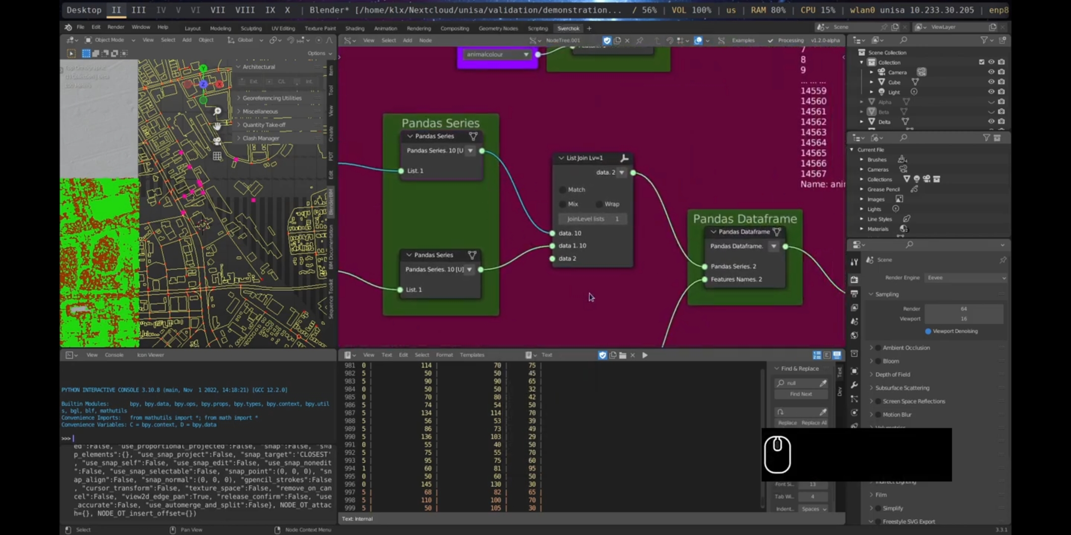
Figure 5.51: Create Dataframe, Port Adelaide
The node Get Sample Dataframe provides access to sample dataframes. These samples, including the Iris, California Price, Diabetes, Digits, and Wine datasets, can be used for demonstration and educational purposes and are well-known in the field of data analytics. The sample datasets were obtained from the Scikit-learn portal26.
5.4.3 Analysis
The analysis process is demonstrated in two parts: Design Analysis and Data Analysis. In the workflow, the analysis process takes as input the output from specific gathering nodes, depending on the analysis task being performed.
5.4.3.1 Design Analysis
The first tool demonstrated in the Design Analysis section is the Dem Attributes tool, which utilises the output from the Read DEM node, DEM Data, to perform topographic analyses of terrain, such as slope and aspect, among others, which are crucial for understanding the geomorphological characteristics of the terrain, for example, in landscape projects. The Dem Attributes node can be combined with the Plot DEM visualisation node to present the results graphically, as shown in Figure 5.52.
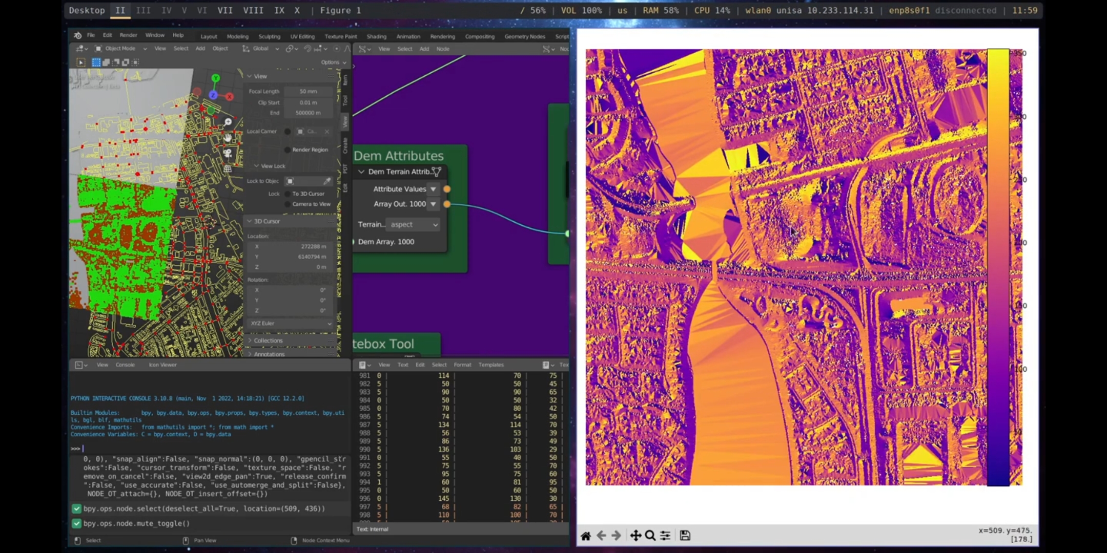
Figure 5.52: Dem Attributes Port Adelaide
The Whitebox Tool node in Sverchok allows access to the Whitebox Tools27, a powerful geospatial analysis tool with over 450 functions for processing various types of geospatial data.
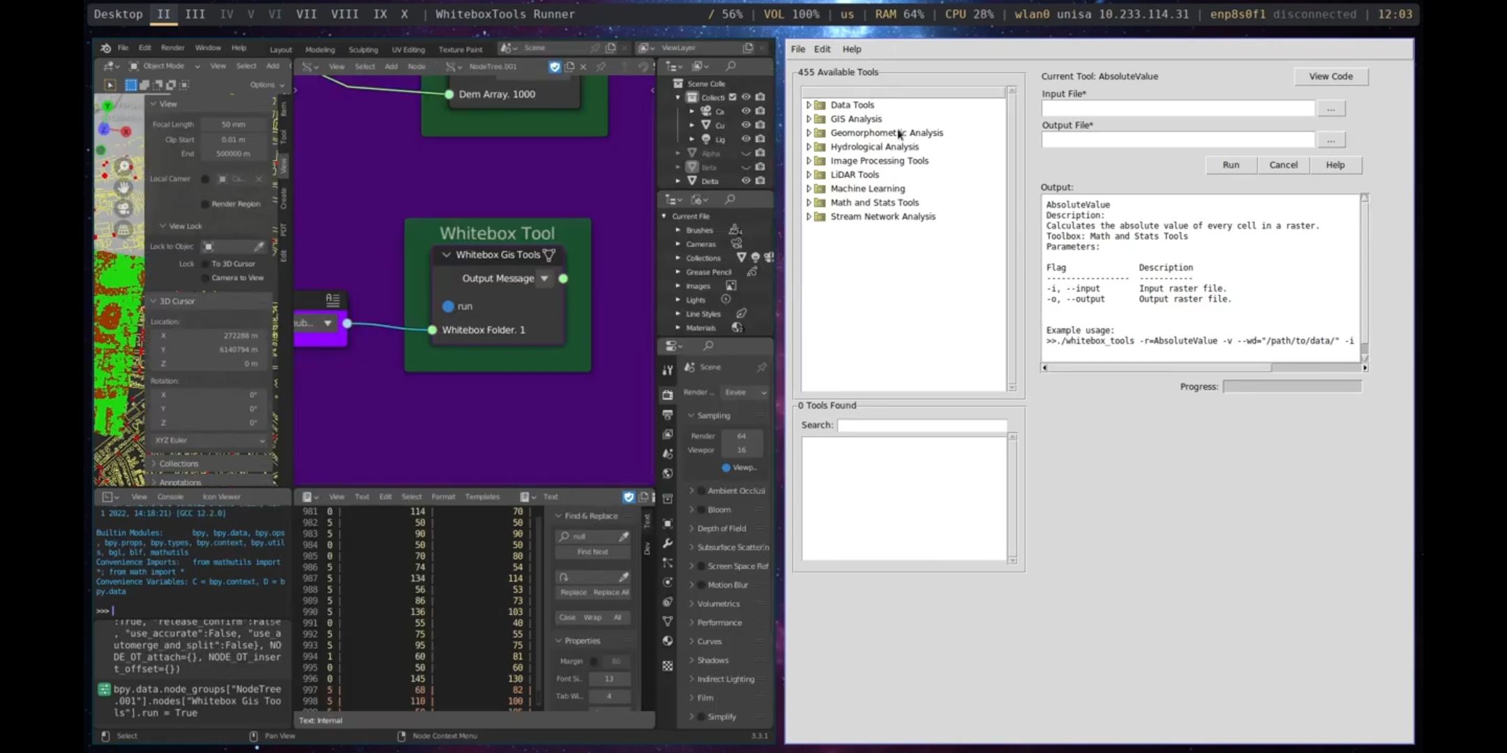
Figure 5.53: Whitebox Tools, Port Adelaide
The Network Analysis node utilises the output of the Load Street Network to perform network analysis. The demonstrated measurements include Closeness Centrality and Between Centrality, which can be used to examine the relationship between street networks and human behaviour (Batty 2013b).
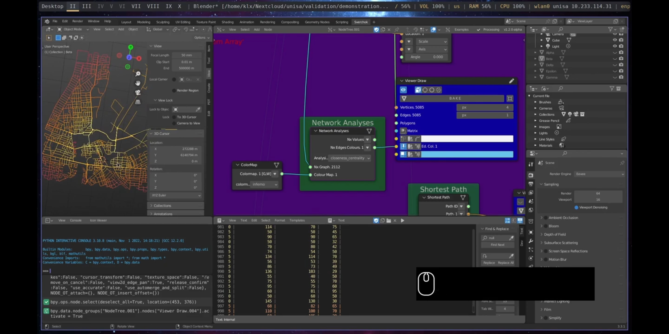
Figure 5.54: Network Analysis, Port Adelaide
The Shortest Path node calculates the shortest path between two points in a street network, providing insight into movement and accessibility within the network.
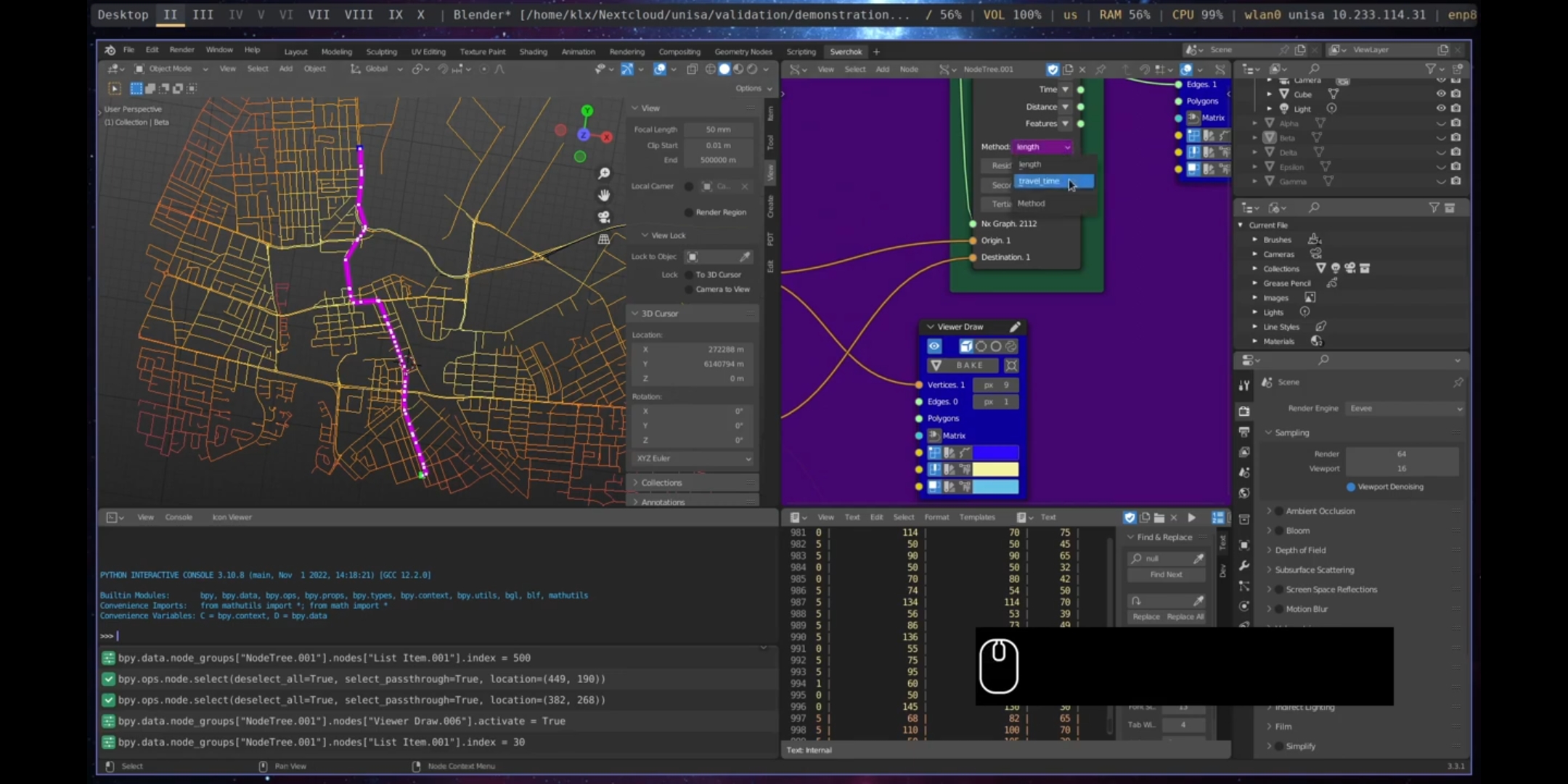
Figure 5.55: Shortest Path, Port Adelaide
5.4.3.2 Analysis Data
The first node in the data analysis process is Data Utils. This node is used to gain an understanding of the characteristics of the data, such as its shape, patterns, and length. This process in data analytics is called exploratory data analysis and is an important step in understanding the dataset and potential relationships it may have.
The demonstration uses a sample dataframe from the Sample Dataframe node to explore its information. The info parameter is used to gather information about the dataset, the head and tail functions are used to get the first and last elements of the dataset, and the describe parameter is used to gather statistical information about the dataset, such as the mean value, percentage distribution, and standard deviation.
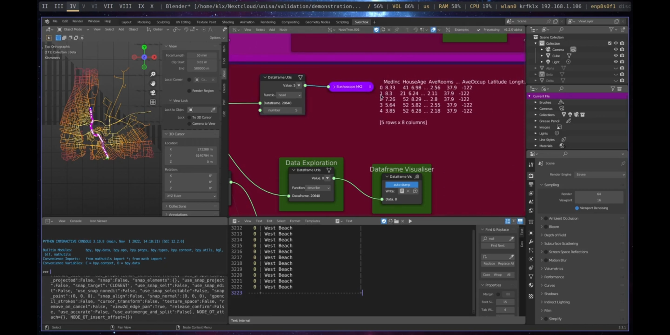
Figure 5.56: Data Utils, Port Adelaide
The visualisation of dataframes using the standard Sverchok output text viewer only partially displays the data, which is why a Dataframe Visualiser node has been implemented to improve dataframe visualisation within Sverchok.
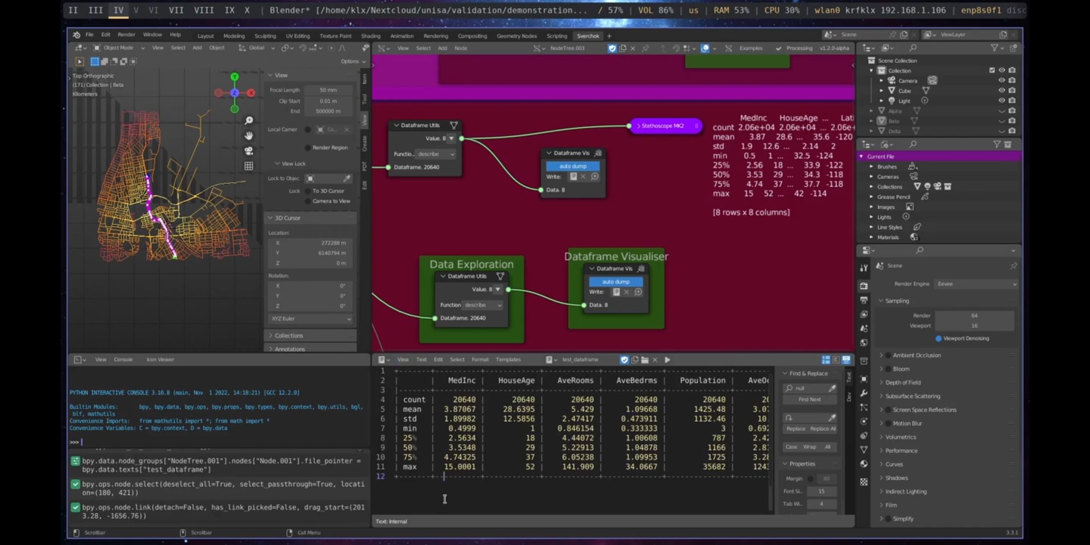
Figure 5.57: Dataframe Visualiser Port Adelaide
The importance of correlations in data-driven urban design lies in their ability to provide insights into the relationships between different variables in a dataset. Correlation is a statistical measure that evaluates the strength and direction of the relationship between two variables. In urban design, correlations can inform design decisions and help designers to identify patterns and trends in the data that may not be immediately obvious. For example, a designer might use correlations to understand how the layout of streets, the availability of green space, and the proximity of amenities affect the overall liveability of a city.
Furthermore, correlations can be used to make predictions about future behaviour. For instance, a designer might predict that people who travel longer distances are more likely to use certain modes of transportation, such as trains or buses, based on the strong correlation between the distance travelled and the mode of transportation used.
The Correlation and Correlation With nodes in Sverchok can be used to perform correlations on a dataset. The Correlation node calculates correlations between all features of the dataframe, while the Correlation With node calculates correlations between a specific feature and the other features of the dataframe. The results of correlations can be visualised using the Plot Heatmap and Seaborn Scatter Plot nodes, as shown in Figures 5.58 and 5.59.
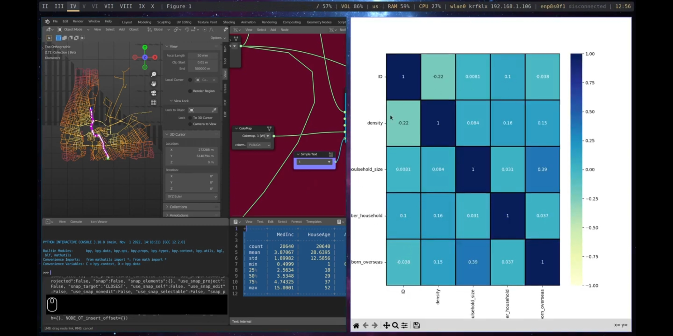
Figure 5.58: Correlation Matrix, Port Adelaide
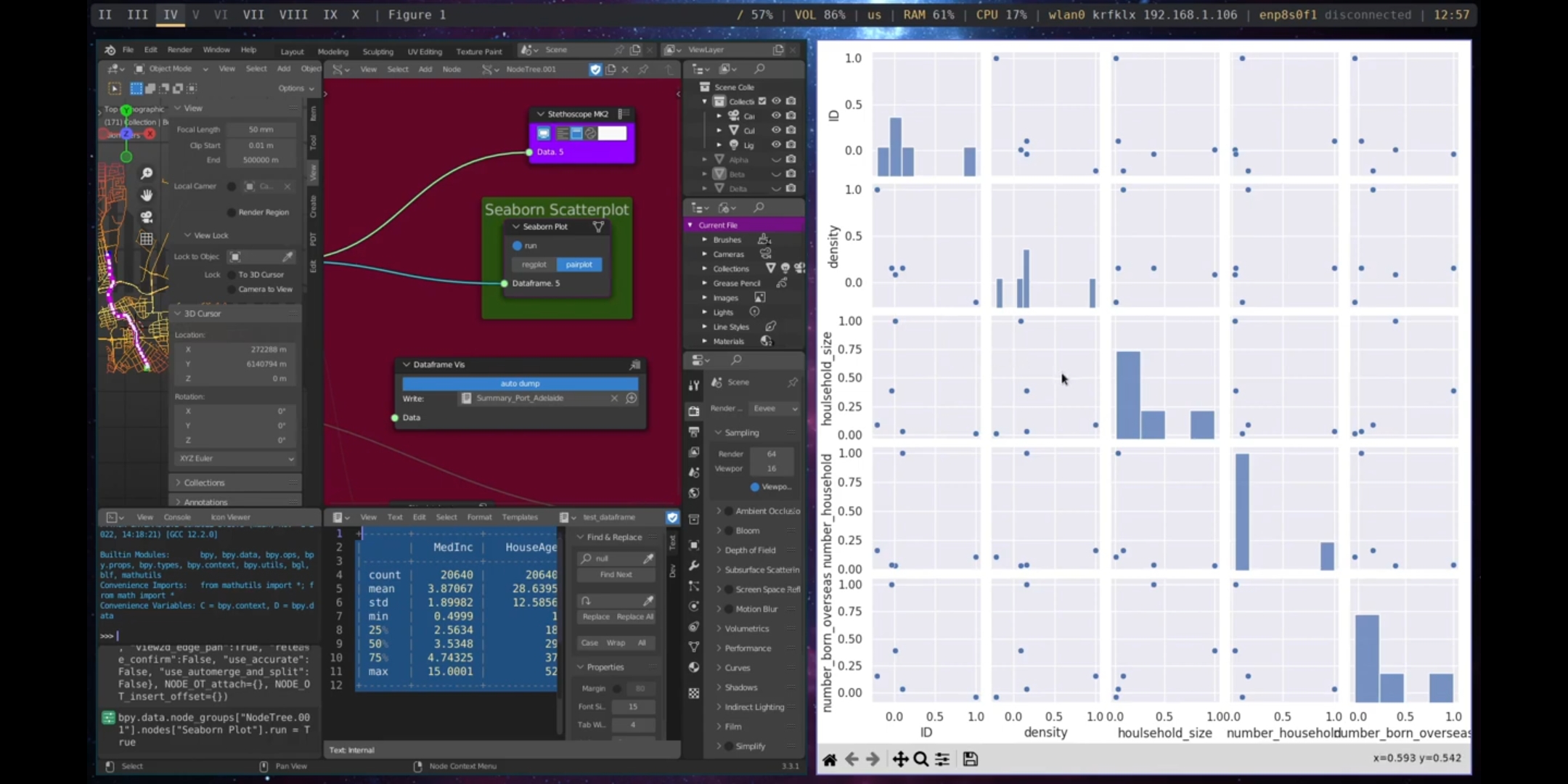
Figure 5.59: Pairplot Correlation, Port Adelaide
Correlation is the first step in determining if there is a strong relationship between one or more features. However, in order to make predictions about how these relationships will behave in the future or under different circumstances, a statistical model must be created. One of the most common models is a linear model. Linear models are statistical techniques used to model the relationship between a dependent variable and one or more independent variables. In data-driven urban design, linear models are important because they enable designers to understand the relationships between variables in a dataset and make predictions about the dependent variable based on the values of the independent variables.
For instance, an urban designer may use a linear model to understand the relationship between the number of people using a transportation system and the mode of transportation they use. By fitting a linear model to the data, the designer can identify the factors that are most strongly associated with the number of people using the transportation system and make predictions about the number of users under different conditions. Linear models are also valuable because they are simple and easy to interpret. The coefficients of the model provide a clear indication of the strength and direction of the relationship between variables. Four nodes are used to create a linear model: Model Selection, Model Fit, Model Predict, and Model Evaluate.
In this demonstration, correlation and linear models were created using datasets from the Australian Bureau of Statistics28 about Port Adelaide. These datasets included population density, household size, number of households, and the born overseas population. The data was processed using pandas nodes within Sverchok.
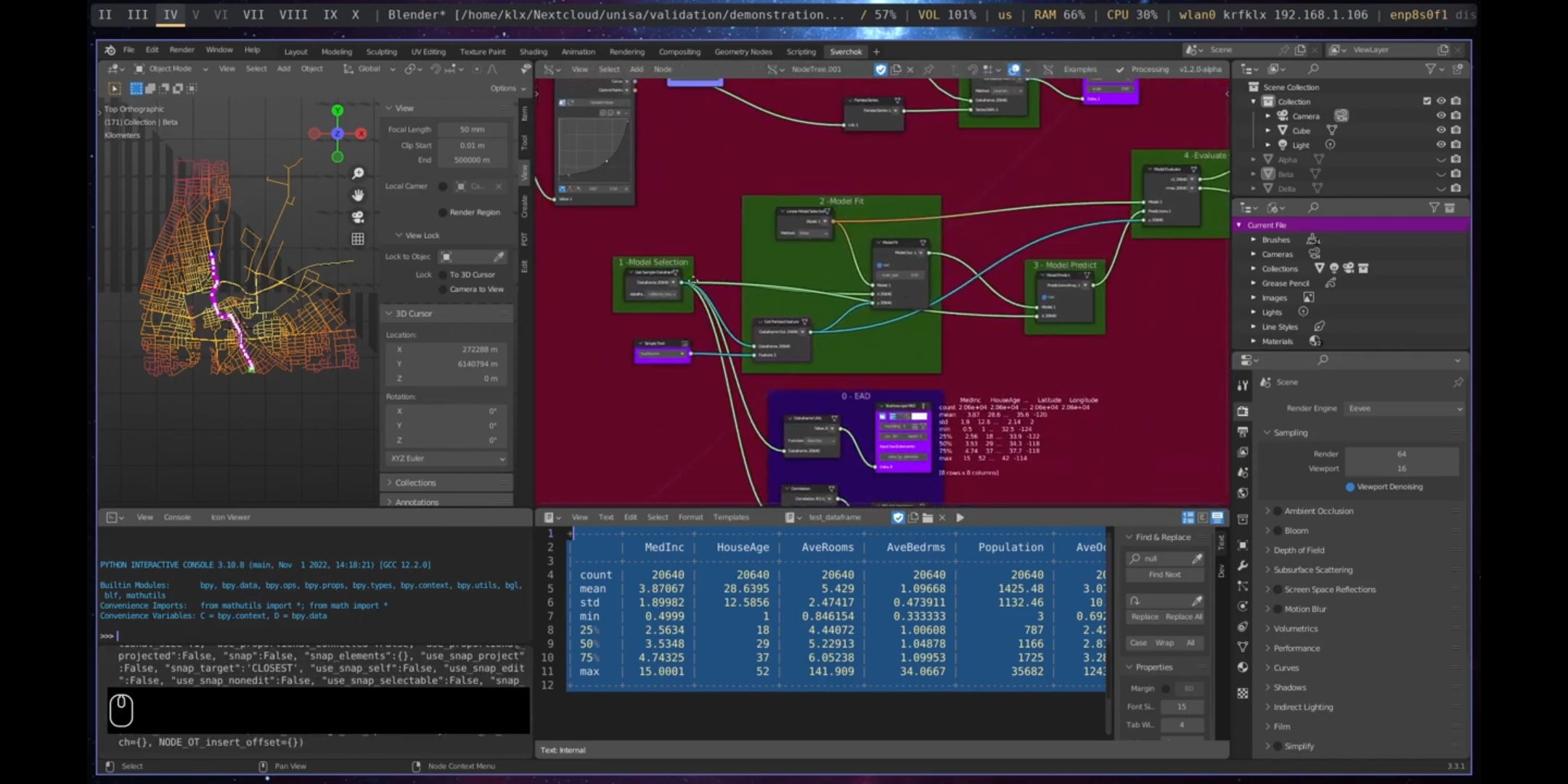
Figure 5.60: Linear Model Creation, Port Adelaide
Finally, the last two nodes demonstrated are Object Detection and Image Segmentation.
Object detection is a computer vision technique that identifies and locates objects in images or video. In data-driven urban design, object detection plays a crucial role in understanding people activity by automatically extracting data about the presence and movements of individuals in public spaces.
For example, an urban designer may use object detection to analyse video footage of a city street and understand how people use the space. The presence and movements of people in the video can provide insights into patterns of activity, and object detection can also be used to track the movements of individuals over time. By analysing video footage captured at different times of day, the designer can understand how the use of the space changes and identify trends in the data, taking into account factors such as weather and events.
Image segmentation, on the other hand, facilitates analysis of urban design features at a granular level. By dividing an image into segments, designers can easily identify and evaluate individual components of the built environment, such as buildings, streets, and parks. This leads to a more nuanced understanding of how different design elements contribute to the overall aesthetic and functional qualities of the streetscape. Previous research has shown that subjective urban design qualities, such as imageability, transparency, complexity, human scale, and enclosure, can be inferred from the analysis of urban elements through image segmentation of streetscape images (Ewing et al. 1997; W. Qiu et al. 2021; Ye et al. 2019).
In the Port Adelaide demonstration, images were gathered using the Download Street Imagery node and segmented using the Image Segmentation node. The outputs generated included images with the segmented areas highlighted and coloured, as well as CSV files containing information on the pixel ratio of elements, categories, id, and category id.
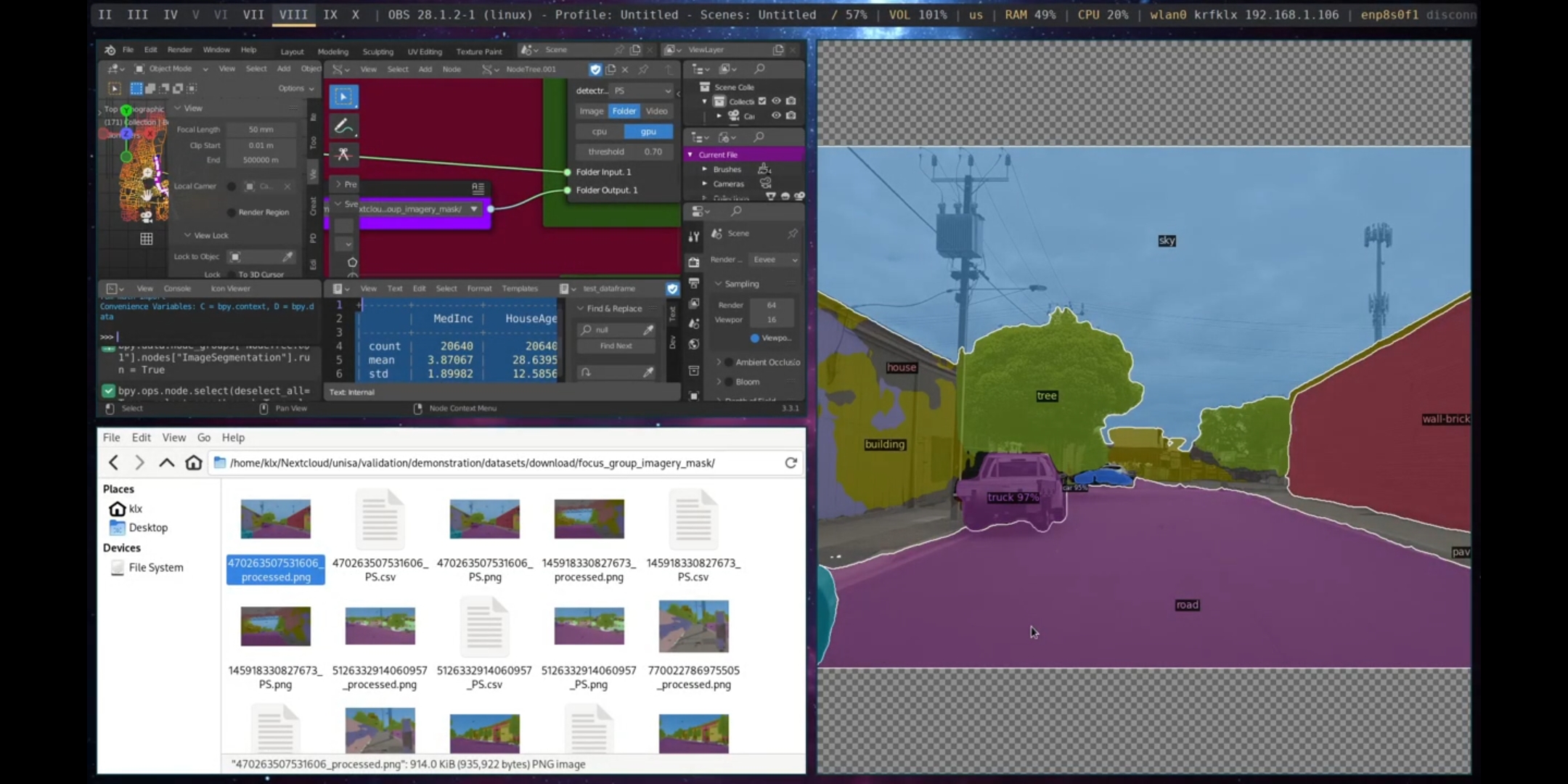
Figure 5.61: Semantic Segmentation, Port Adelaide
5.4.4 Visualisation
Data visualisation is a critical component of evidence-based processes in data-driven urban design, as it enables the effective presentation and communication of complex datasets in a manner that is easily understood by a broad audience. There are several reasons why data visualisation is important in this context.
Firstly, it helps with the analysis and interpretation of data by presenting it concisely. Graphical representations, such as charts, maps, and diagrams, allow designers to easily identify patterns, trends, and relationships within the data and use this information to inform design decisions.
Secondly, data visualisation enables effective communication of findings to a diverse group of stakeholders, including planners, policymakers, and community members. By presenting data in an accessible and visually appealing manner, designers can more effectively communicate their findings and recommendations to these groups, leading to increased collaboration and engagement in the design process.
Finally, data visualisation helps to ensure transparency and accountability in the design process. By presenting data in a clear and easily understandable manner, designers can demonstrate the evidence and reasoning behind their decisions and allow for greater scrutiny and evaluation by others, creating trust and confidence in the design process, and ensuring that the design solutions are based on robust evidence.
To improve the integration and simplicity of visualisation methods, iterative dashboards have been developed as a strategy. Dashboards provide a centralised and interactive platform for accessing, analysing, and visualising data, and can make it easier for designers to communicate their findings and recommendations to stakeholders.
In the Port Adelaide demonstration, data and design visualisation tools were integrated and presented as a single dashboard that includes maps, graphs, dataframes, and text. This method can be used to support and build narratives for developed projects and assist with collaboration and stakeholder engagement.
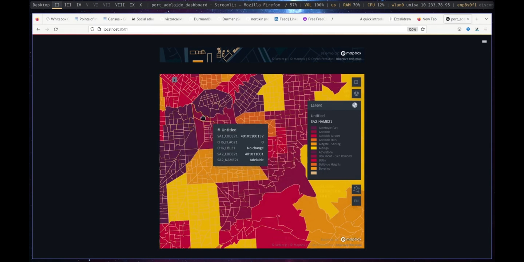
Figure 5.62: Dashboard Map, Port Adelaide
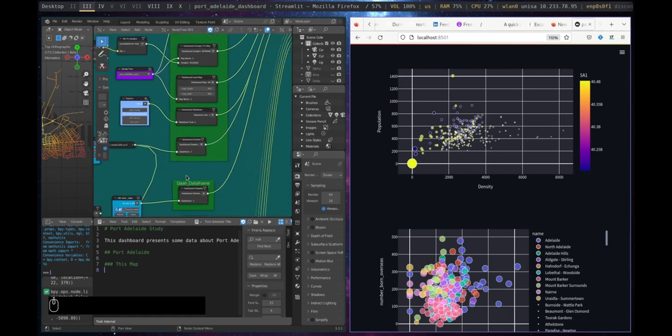
Figure 5.63: Dashboard Plot Port Adelaide
5.5 Conclusion
This chapter presented the development of a computational prototype and demonstrated it through a scenario. The prototype provides an integrated environment to assist data-driven computational urban design processes, including data, design, and supporting tools across design steps and data procedures. This integration was built through seven cores, enabling computational smart technologies (GIS, Data Analytics, Spatial Data Analytics, Web Services, Image Classification, Geometry Processing, and Immersive Technologies) that can potentially address multiple urban design dimensions. Moreover, the computational toolkit was developed entirely from Free and Open-Source libraries and services, considering an holistic socio-political understanding of the digital toolmaking process in relation to future smart cities, promoting community-driven development and the democratisation of access to data-driven urban design tools.
The demonstration was effective in its purpose of presenting the distinct functionalities of the computational toolkit, as well as its usability in a real-world scenario, providing options for integration of design and data across the seven core enabling technologies.
The following chapter presents the research validation process, which was conducted through a focus group comprising a balance of both traditional and data-driven designers.
The curvature diagram was adapted from ArchGIS Repository Center↩︎
Further description: https://scikit-learn.org/stable/modules/linear_model.html↩︎
Scenario Demonstration link: https://youtu.be/lTRNIa2PwhQ↩︎
MEGA-POLIS:https://github.com/victorcalixto/mega-polis ↩︎
Blender: https://www.blender.org/↩︎
Sverchok: https://github.com/nortikin/sverchok↩︎
OpenStreetmap: https://www.openstreetmap.org/↩︎
Mapillary: https://www.mapillary.com/app/↩︎
Port Adelaide Historical Photos: https://data.sa.gov.au/data/dataset/local-history-photo-collection↩︎
Pandas: https://pandas.pydata.org/↩︎
Scikit-learn: https://scikit-learn.org/stable/datasets/toy_dataset.html↩︎
Whitebox Tools: https://www.whiteboxgeo.com/↩︎
Australian Bureau of Statistics: https://www.abs.gov.au/census↩︎