Catenary Form-Finding
The Catenary form-finding is an interesting script that has its origins in Gaudi’s chain models that he developed for the Sagrada Familia cathedral. In these models, Gaudi explored structural plasticity using funicular forms (or catenary forms) that are dominated by axial forces (compression and tension forces). These models are efficient and elegant active structural forms based on simple forces. Gaudi’s models use a chain divided into segments that hangs scaled weights representing the forces. The chain curvature is under tension, creating a funicular form. If generated for is flipped, it results a curvature optimised to resist to compression. The catenary form is stable and optimises material usage.
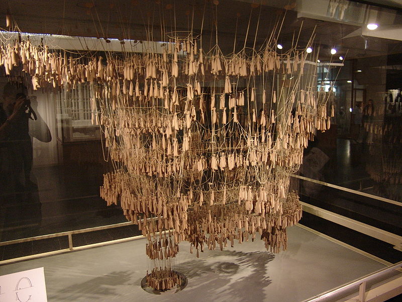
Another architect that explored this theme was Heinz Isler. Isler’s experiments are free form physical models that use a fabric surface with a plaster formula. This method is called hanging cloth reversed.
Nowadays, several Grasshopper scripts simulate this process using Kangaroo physics. It is one of the most loved scripts that I have ever seen.
In this tutorial, we recreate this process in Blender/Sverchok using Pulga. Pulga, similar to Kangaroo for Grasshopper, is a physical simulation solver based on particles.

So, let’s do it.
Creating a Plane and Defining Structural Supports.
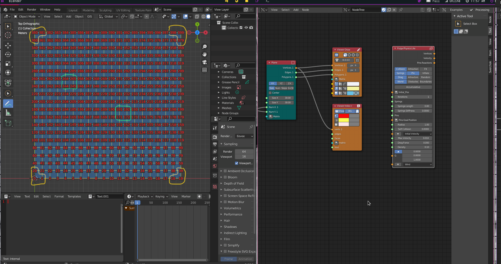
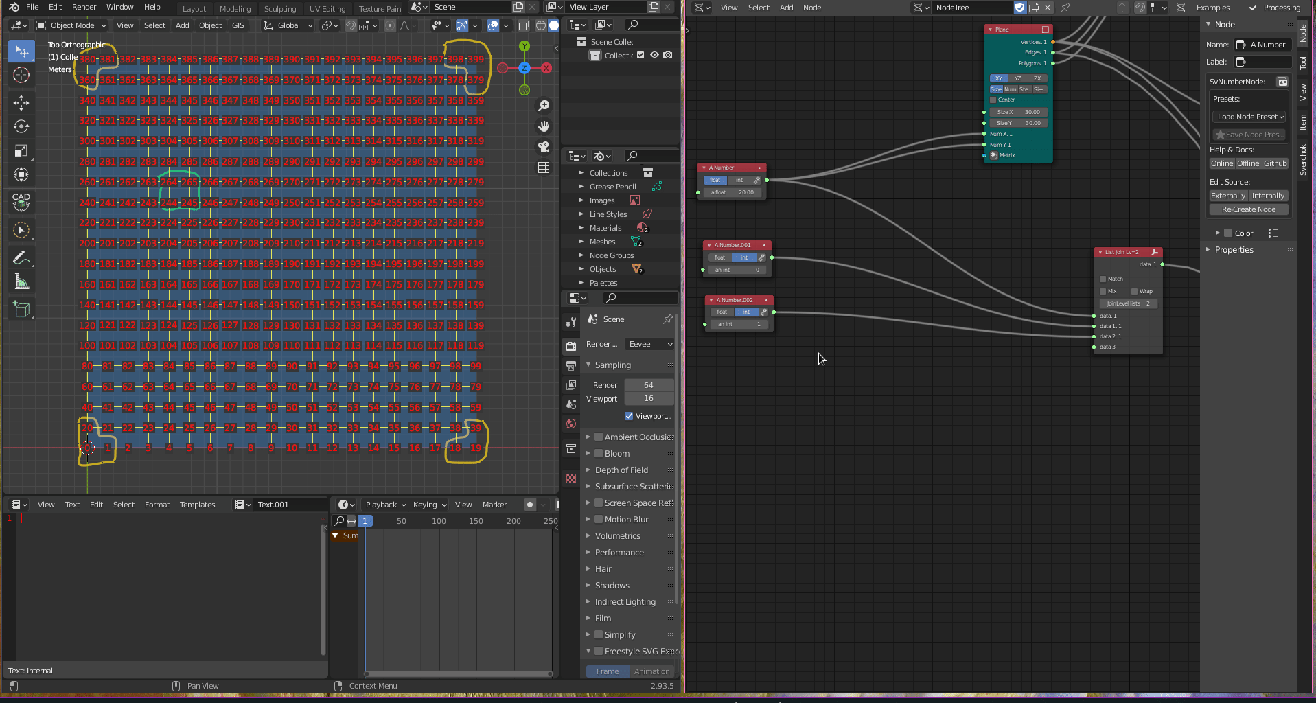
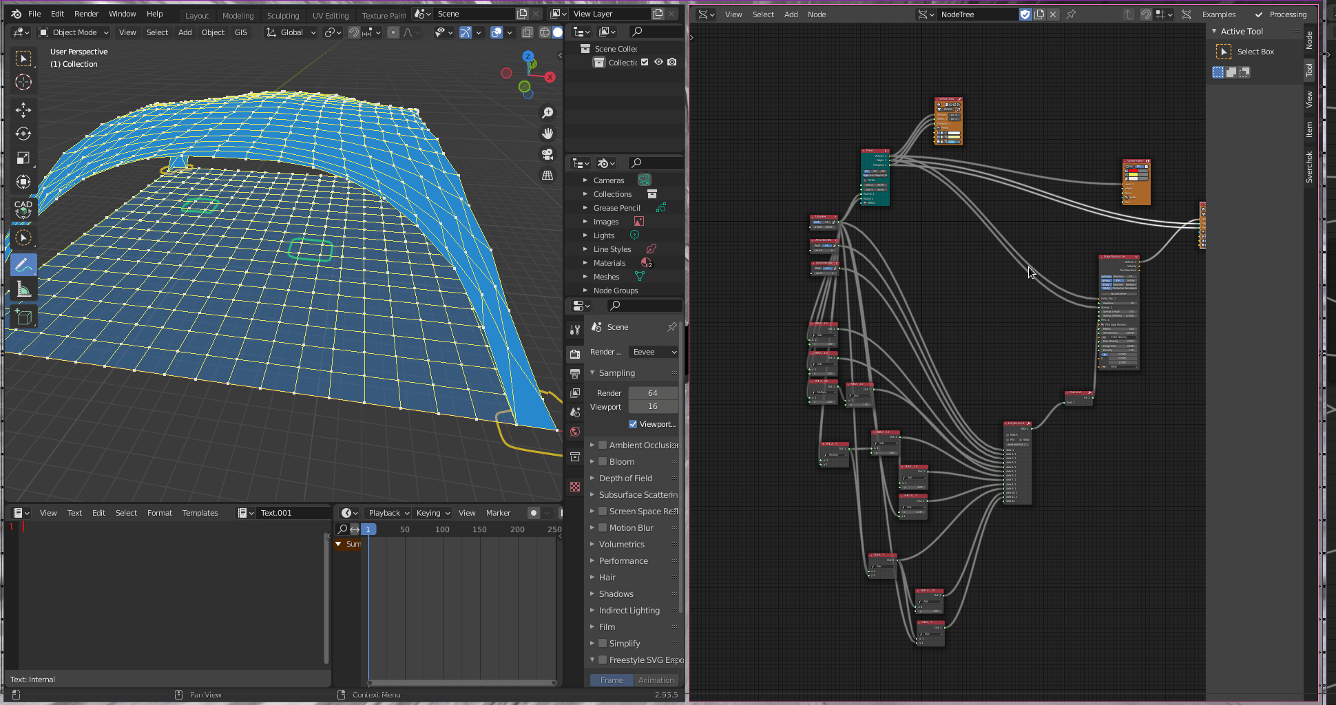
First, we create a Plane(Generator-> Plane). We change the values from Size X and Size Y to 30. Then, we use an A number(Number -> A Number) node to define the values for Num X and Num Y, which is the number of divisions of the plane. We use a Viewer Draw (Viz -> Viewer Draw to visualise the plane.
In a notation form these operations and values can be defined as follow:
Plane { XY; Size; Size X: 30; Size Y: 30}
A Number {Int; an int: 20} * I did not change from float to int in the example, but using int it is more efficient.
Operations
(A Number (int) [->]) -> (Plane [Num X <-])
(A Number (int) [->]) -> (Plane [Num Y <-])
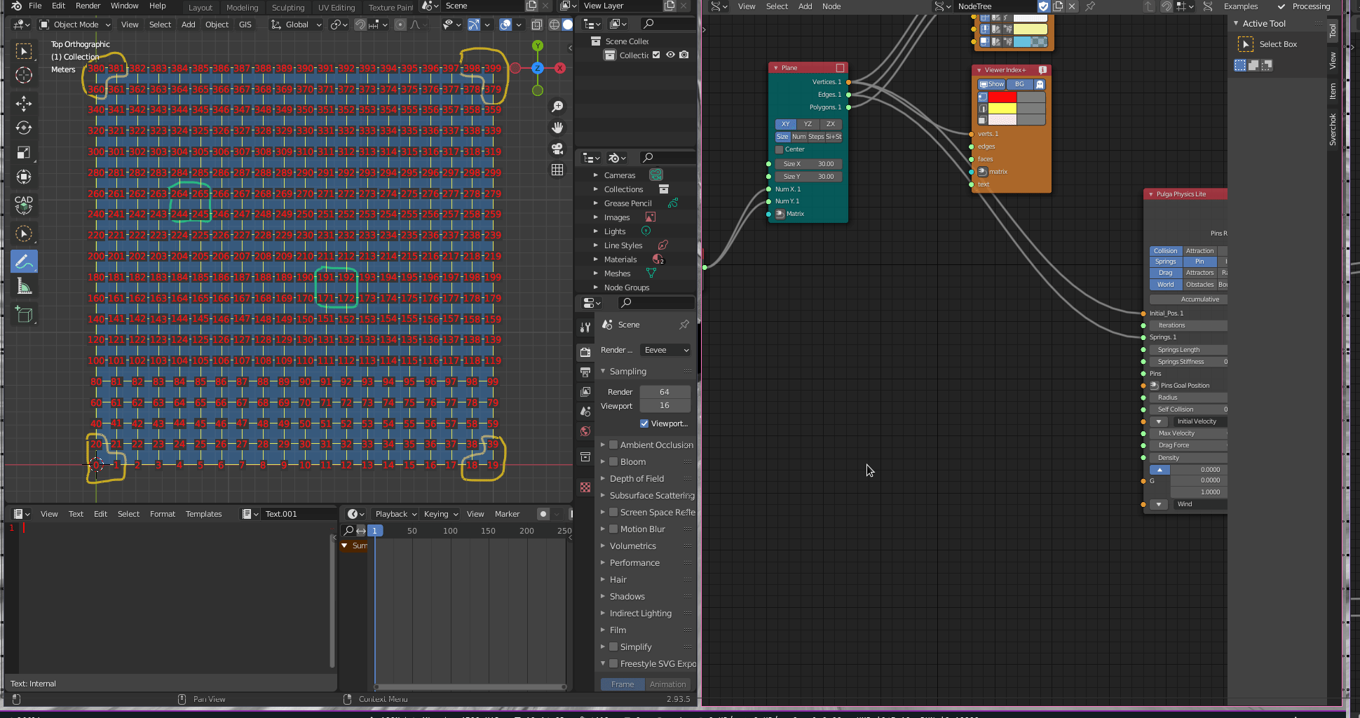
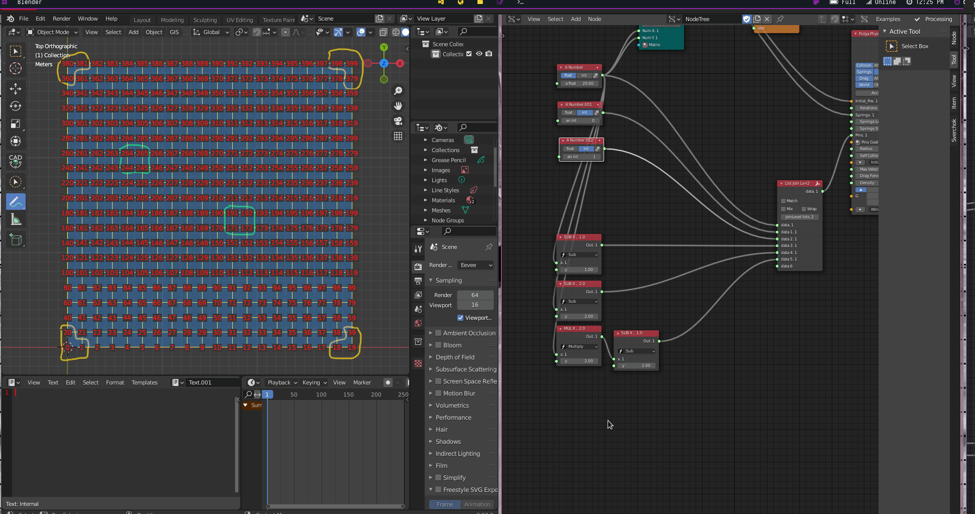
To set up structural supports (or pins) for the shell, we need to first understand the indexes of each vertex of the structure. We use the Viewer Index +(Viz -> Viewer Index +) to access the indexes.
Viewer Index + {Show; BG}
Operations
(Plane [Vertices ->]) -> (Viewer Index + [verts <-])
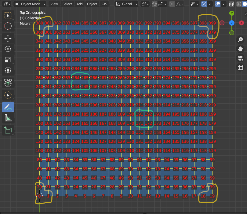
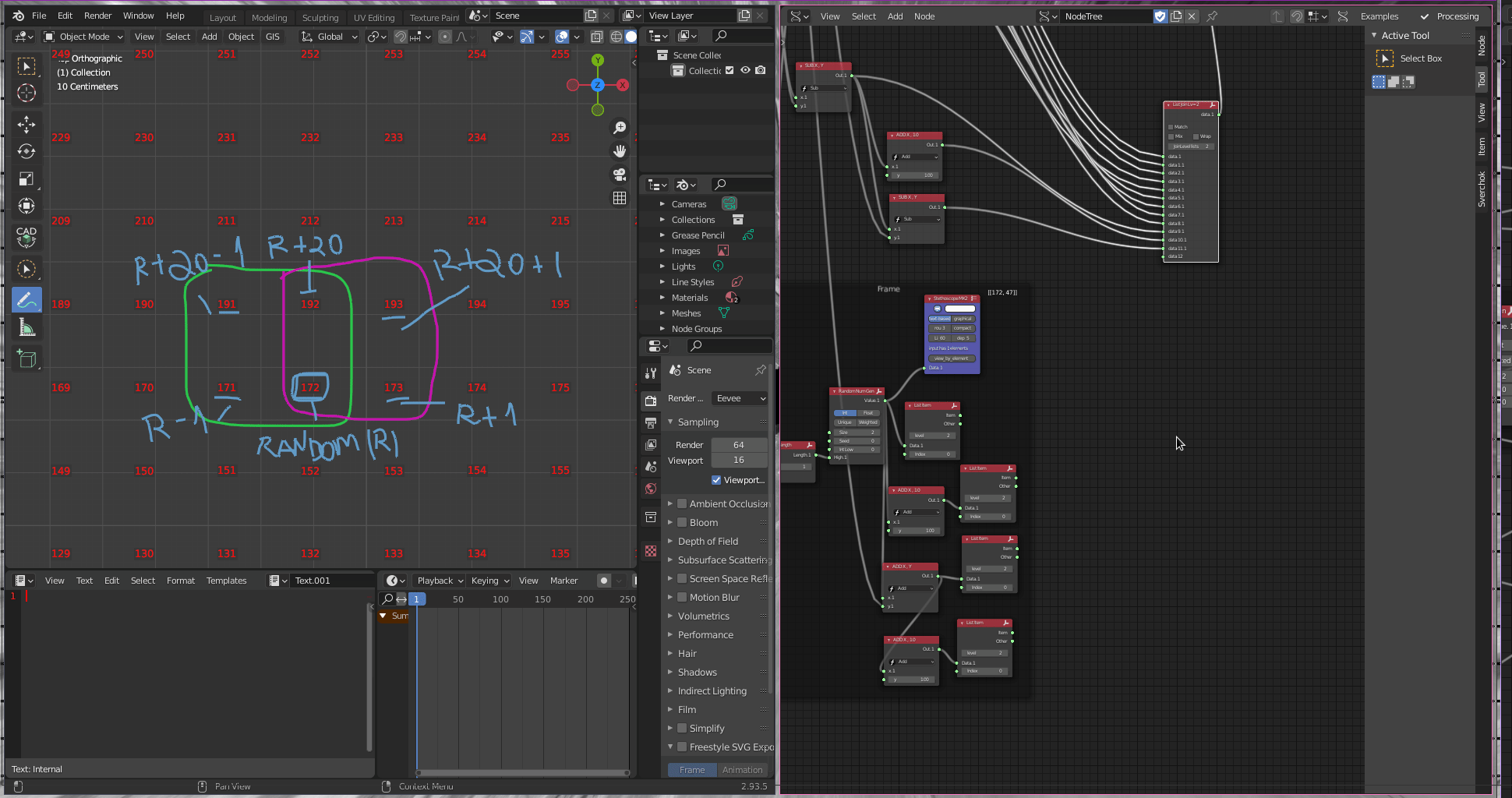
Let’s have a look at the vertices of the structure. If we want to have a stable structure, we can start humble and cautious by selecting vertices from the extremities (represented in the image in yellow ).
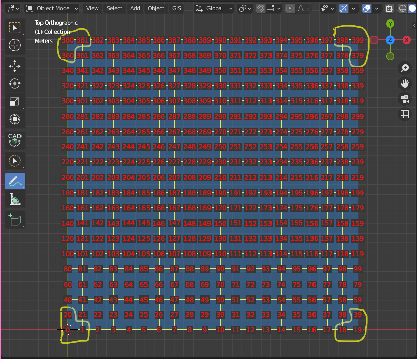
But, to make it more dynamic, we can define two structural supports that randomically change position based on a seed value (represented in the image in cian ).
Before starting to create the vertices, we can set up Pulga Physics Solver to receive the pin indexes. We use a Pulga Physics Lite(Pulga Physics -> Pulga Physics Lite) node. Then we connect the Plane vertices and edges to Pulga Physics Lite
Pulga Physics Lite {Collisions; Springs, Drag, World, Pin; Gravity: Z : 1}
Operations
(Plane [vertices ->]) -> (Pulga Physics Lite [Initial_pos <-])
(Plane [edges ->]) -> (Pulga Physics Lite [Springs <-])
Structural Supports from the Extremities
Now we can start to define the pins. First, let’s start with the vertices from the extremities.
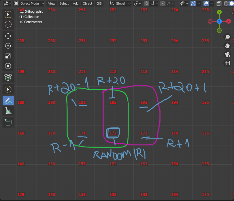
To access the vertices from the extremities, we need the indexes [0,1,18,19,39,360,379,380,381,398,399]. We could type these numbers to set the pins, but if we decide to change the planes divisions, we have to rewrite the indexes. A better approach is to parametrically define these vertices based on the values that we already have.
For the first support [0,1,20], we can use an A Number (1) node for 0 and another A Number (2) node for 1, because no matters how many divisions the structure has, if it follows the same logic, the 0 and 1 will be included as indexes. Then, we can use the first A number that defines the number of divisions in the plane as our index number 20. If we decide to change the number of divisions, this index will be associated with this number. We create a List Join node to connect these values into a single list, then we connect the List Join output into the Pins input of the Pulga Physics Lite node.
List Join {JoinLevel list: 2}
Operations
(A Number [->]) -> (List Join [data 1 <-])
(A Number (1) [->]) -> (List Join [data 1.1 <-])
(A Number (2) [->]) -> (List Join [data 2.1 <-])
(List Join [data ->]) -> (Pulga Physics Lite [Pins <-])
For the second support [18,19,39], we can establish the following relation:
index 19 = number of plane divisions -1
index 18 = number of plane divisions -2
index 39 = (number of plane divisions * 2)-1
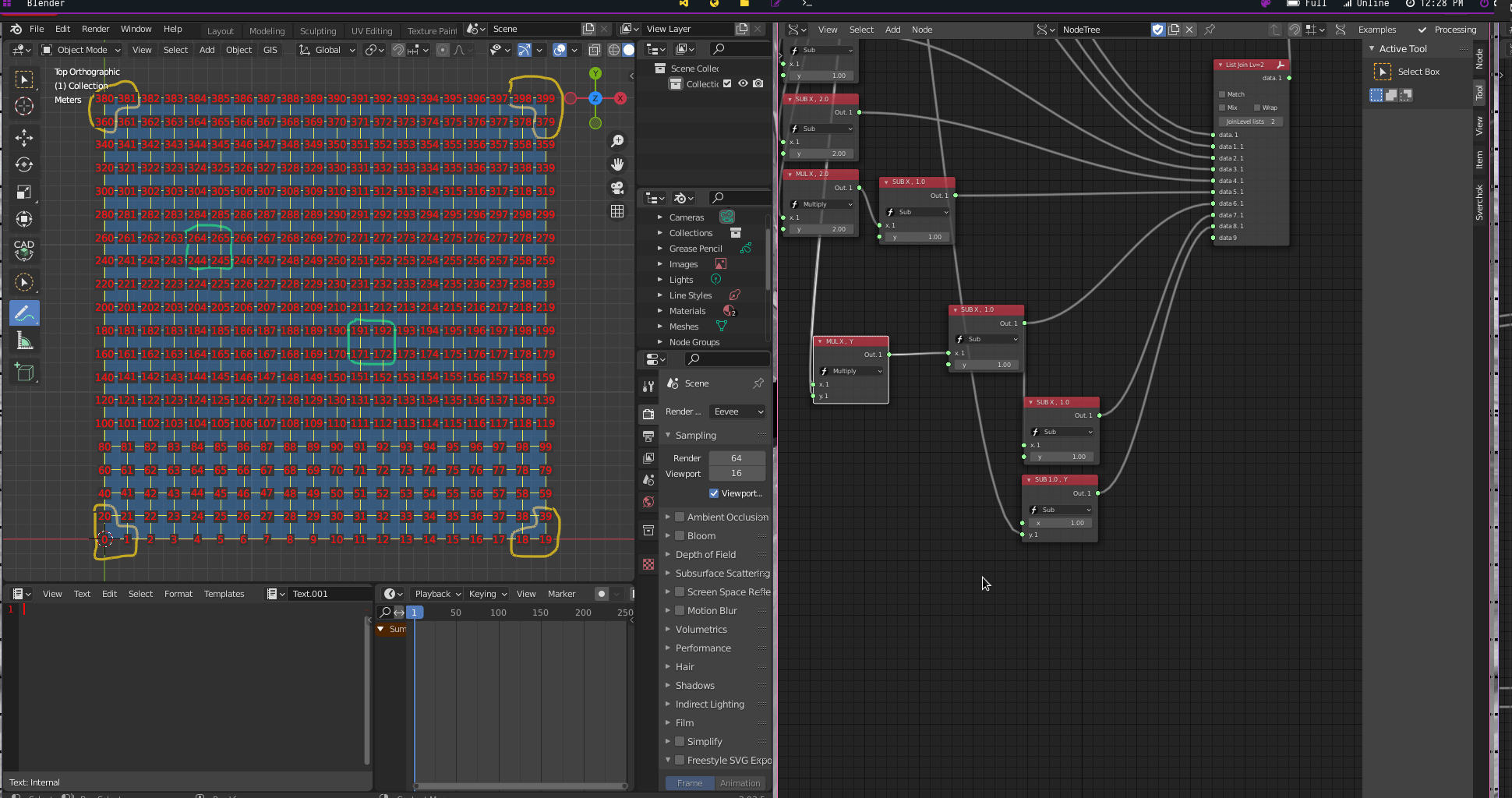
We use Scalar Math (Sub, Multiply)(Number -> Scalar Math) nodes to create these operations.
Scalar Math {Sub; y : 1}
Scalar Math (1) {Sub; y : 2}
Scalar Math (2) {Multiply; y : 2}
Scalar Math (3) {Sub; y : 1}
Operations
(A Number [->]) -> (Scalar Math [x 1 <-])
(A Number [->]) -> (Scalar Math (1)[x 1 <-])
(A Number [->]) -> (Scalar Math (2)[x 1 <-])
(A Number [->]) -> (Scalar Math (3)[x 1 <-])
(Scalar Math [Out ->]) -> (List Join [data 3.1 <-])
(Scalar Math (1) [Out ->]) -> (List Join [data 4.1 <-])
(Scalar Math (2) [Out ->]) -> (Scalar Math (3) [x <-])
(Scalar Math (3) [Out ->]) -> (List Join [data 5.1 <-])
For the third support [379,398,399]:
index 399 = (number of plane divisions * number of plane divisions)-1
index 398 = (number of plane divisions * number of plane divisions)-2
index 379 = ((number of plane divisions * number of plane divisions)-number of plane divisions)-1
We use the Scalar Math node again to create these operations.
Scalar Math (4) {Multiply; x: A Number; y: A Number}
Scalar Math (5) {Sub; y: 1}
Scalar Math (6) {Sub; y: 1}
Scalar Math (7) {Sub; y: A Number}
Scalar Math (8) {Sub; y: 1}
Operations
(A Number [->]) -> (Scalar Math (4) [x,y <-])
(Scalar Math (4)[Out ->]) -> (Scalar Math (5) [x <-])
(Scalar Math (5)[Out ->]) -> (Scalar Math (6) [x <-])
(A Number [->]) -> (Scalar Math (7) [y <-])
(Scalar Math (4)[Out ->]) -> (Scalar Math (7) [x <-])
(Scalar Math (7)[Out ->]) -> (Scalar Math (8) [x <-])
(Scalar Math (5) [Out ->]) -> (List Join [data 6.1 <-])
(Scalar Math (6) [Out ->]) -> (List Join [data 7.1 <-])
(Scalar Math (8) [Out ->]) -> (List Join [data 8.1 <-])
For the fourth support [360,380,381]:
index 380 = (number of plane divisions * number of plane divisions)-number of plane divisions
index 381 = ((number of plane divisions * number of plane divisions)-number of plane divisions)+1
index 360 = ((number of plane divisions * number of plane divisions)-number of plane divisions)-number of plane divisions)
The Scalar Math operations:
Scalar Math (9) {Sub; x: Scalar Math (4); y: A Number}
Scalar Math (10) {Add; x: Scalar Math (9); y: 1)
Scalar Math (11) {Sub; x: Scalar Math (9); y: A Number}
Operations
(Scalar Math (4)[Out ->]) -> (Scalar Math (9)[x <-])
(A Number [->]) -> (Scalar Math (9)[y <-])
(Scalar Math (9)[Out ->]) -> (Scalar Math (10)[x <-])
(Scalar Math (9)[Out ->]) -> (Scalar Math (11)[x <-])
(A Number [->]) -> (Scalar Math (11)[y <-])
(Scalar Math (9) [Out ->]) -> (List Join [data 9.1 <-])
(Scalar Math (10) [Out ->]) -> (List Join [data 10.1 <-])
(Scalar Math (11) [Out ->]) -> (List Join [data 11.1 <-])
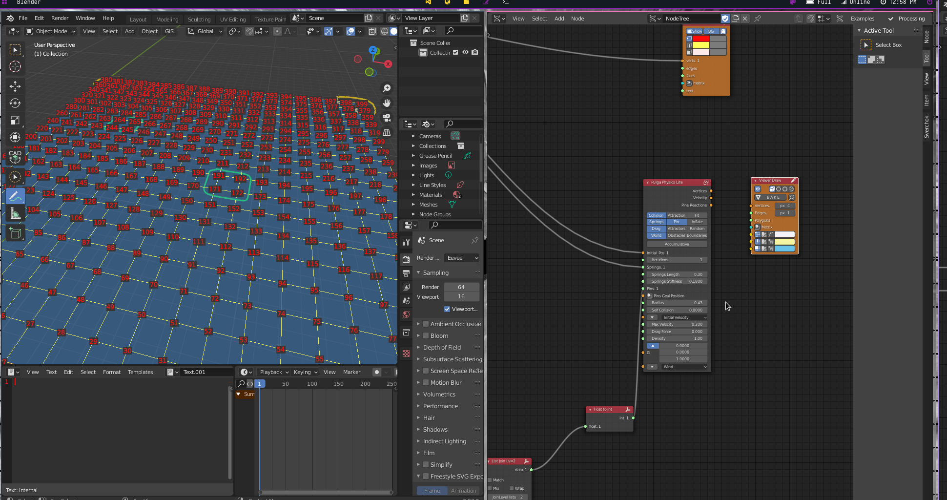
We need to convert the values from the List Join node into integer values. We use a Float to Int(Number -> Float to int) node.
Operations
(List Join [Out ->]) -> (Float to Int [float <-])
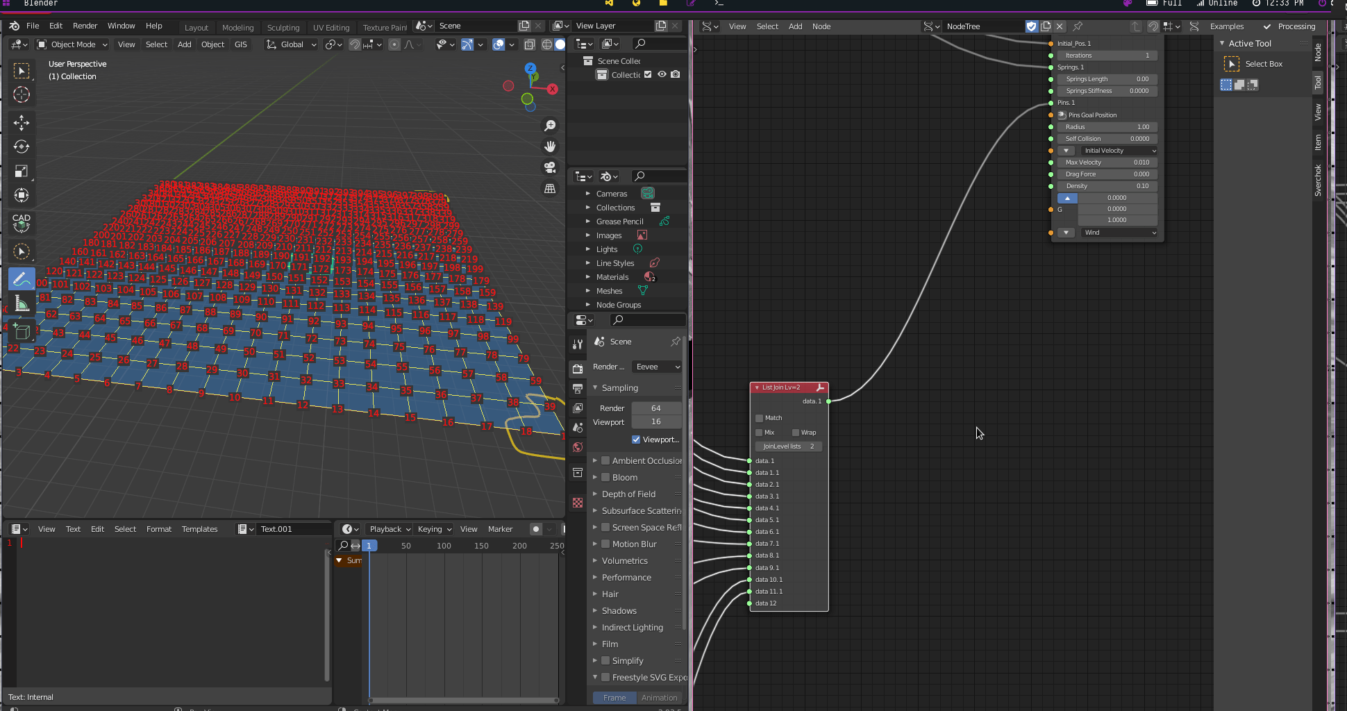
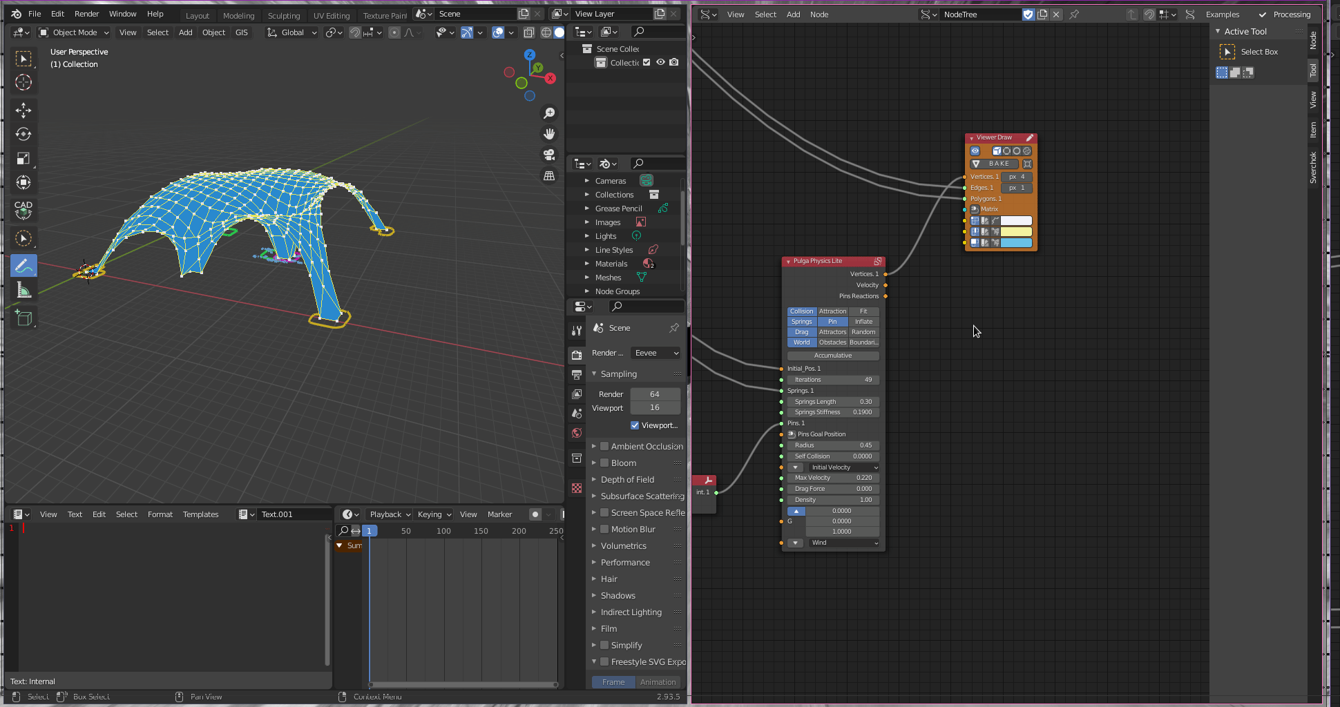
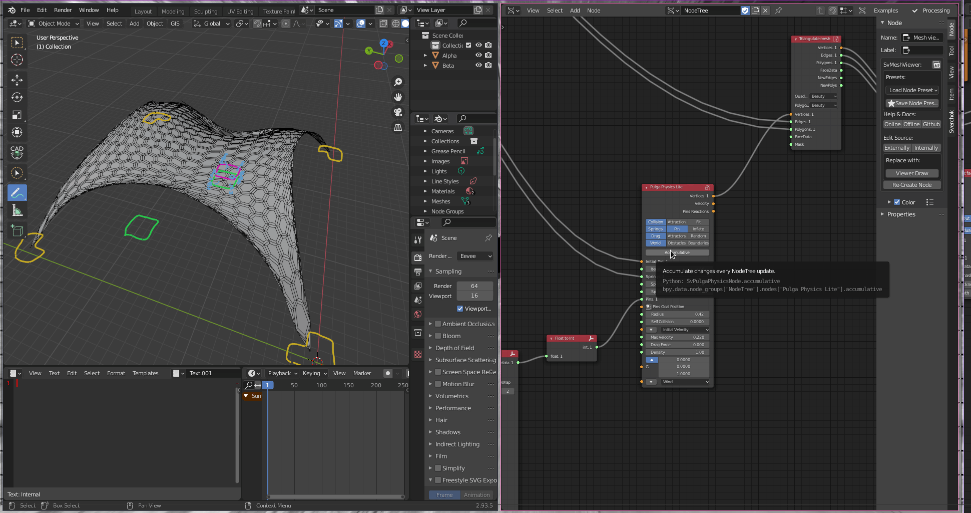
It is time to visualise the shell. We use a Viewer Draw (1) connecting Pulga Physics Lite vertices and Plane edges and polygons outputs. Then, we change the parameters of Pulga Physics Lite, incrementing iterations one by one.
Pulga Physics Lite {Collisions; Springs; Drag; World; Pin; Gravity: Z : 1; Spring Length: 0.30; Spring Stifiness: 0.19; Radious: 0.45; Max Velocity: 0.22; Iterations: 43}
Operations
(Pulga Physics Lite [Vertices ->]) -> (Viewer Draw (1)[Vertices <-])
(Plane [edges ->]) -> (Viewer Draw (1)[Edges <-])
(Plane [Polygons ->]) -> (Viewer Draw (1)[Faces <-])
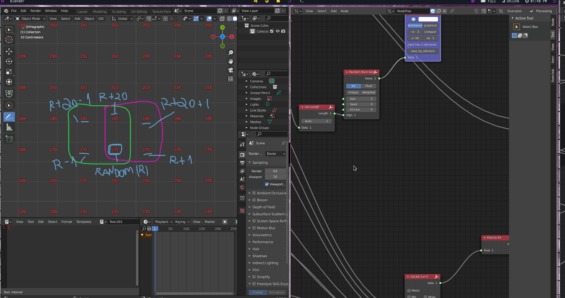
Random Structural Supports
Now we need to create random structural supports. First, we use a List Length(List -> List Main -> List Length node to count the vertices of the plane. Then, we use a Random Num Gen(Number -> Random Num Gen) to generate the two random numbers that will define the structural supports.
Random Num Gen {Int; Size: 2}
Operations
Plane [vertices ->]) -> (List Length [data <-])
(List Length [Length ->]) -> (Random Num Gen [Int High <-])
There are two methods for structural supports creation that follows the same logic:
Method 1
Random Number
Random Number + 1
Random Number + Number of Plane Divisions
Random Number + Number of Plane Divisions + 1
Method 2
Random Number
Random Number - 1
Random Number + Number of Plane Divisions
Random Number + Number of Plane Divisions - 1
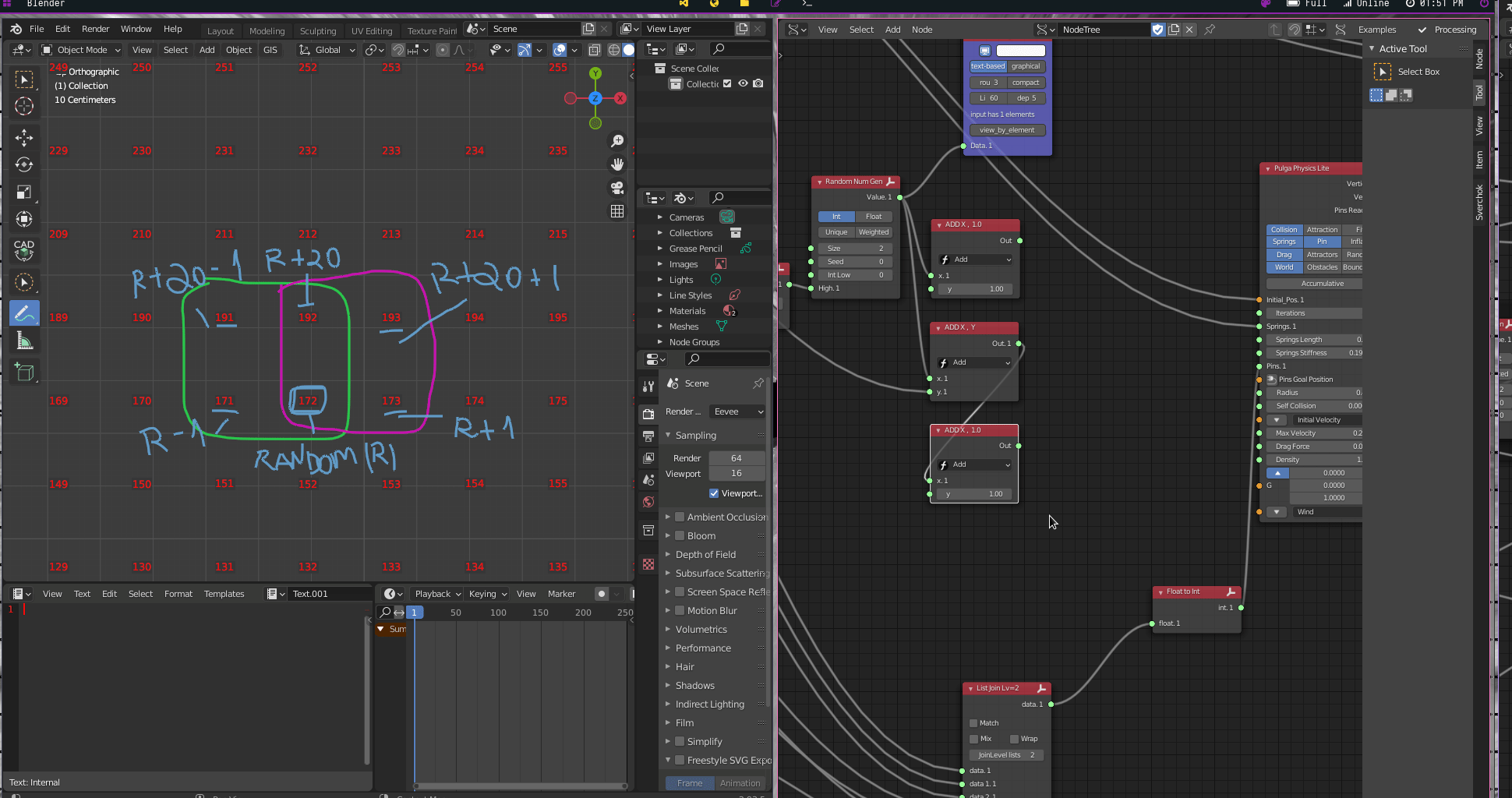
We use Method 1 in this example, using the Scalar Math to create these operations:
Scalar Math (12) {Add; x: Random Num Gen; y: 1}
Scalar Math (13) {Add; x: Random Num Gen ; y: A Number)
Scalar Math (14) {Sub; x: Scalar Math (13); y: 1}
Operations
(Random Num Gen [Value ->]) -> (Scalar Math (12,13) [x <-])
(A Number [->]) -> (Scalar Math (13) [y <-])
(Scalar Math (13) [Out ->]) -> (Scalar Math (14) [x <-])
We use a List Item(List -> List Struct -> List Item) node for each Random parameter stabilised before. It will divide the random values–that are composed of a list of two values–in a single number.
(Random Num Gen [Value ->]) -> (List Item [Data <-])
(Scalar Math (12) [Value ->]) -> (List Item (1)[Data <-])
(Scalar Math (13) [Value ->]) -> (List Item (2)[Data <-])
(Scalar Math (14) [Value ->]) -> (List Item (3)[Data <-])
Then, we connect those List Item nodes into the List Join node.
(List Item [Item ->]) -> (List Join [data 12.1 <-])
(List Item [Other ->]) -> (List Join [data 13.1 <-])
(List Item (1) [Item ->]) -> (List Join [data 14.1 <-])
(List Item (1) [Other ->]) -> (List Join [data 15.1 <-])
(List Item (2) [Item ->]) -> (List Join [data 16.1 <-])
(List Item (2) [Other ->]) -> (List Join [data 17.1 <-])
(List Item (3) [Item ->]) -> (List Join [data 18.1 <-])
(List Item (3) [Other ->]) -> (List Join [data 19.1 <-])
Creating Panels
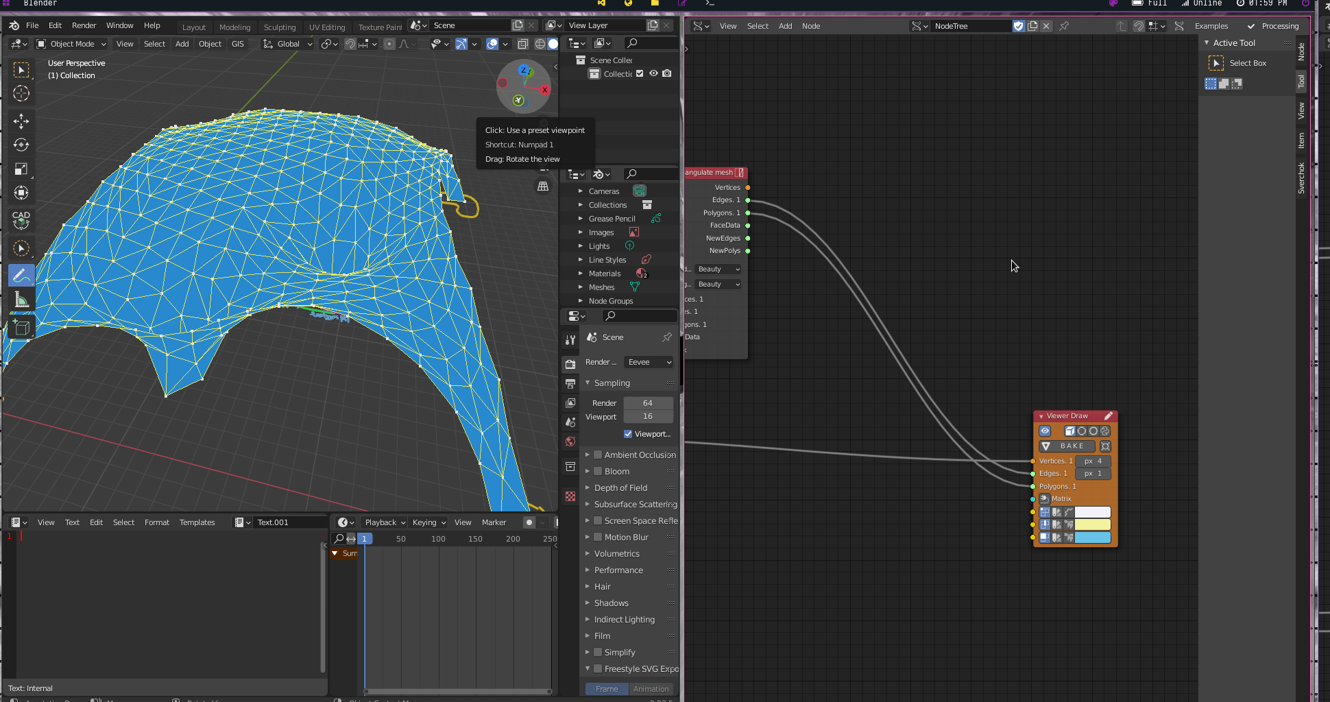
Now we create panels. First, we use the Triangulate Mesh(Modifiers -> Modifiers Change -> Triangulate Mesh). We connect the vertices from Pulga Physics Lite and edges and polygons from Plane.
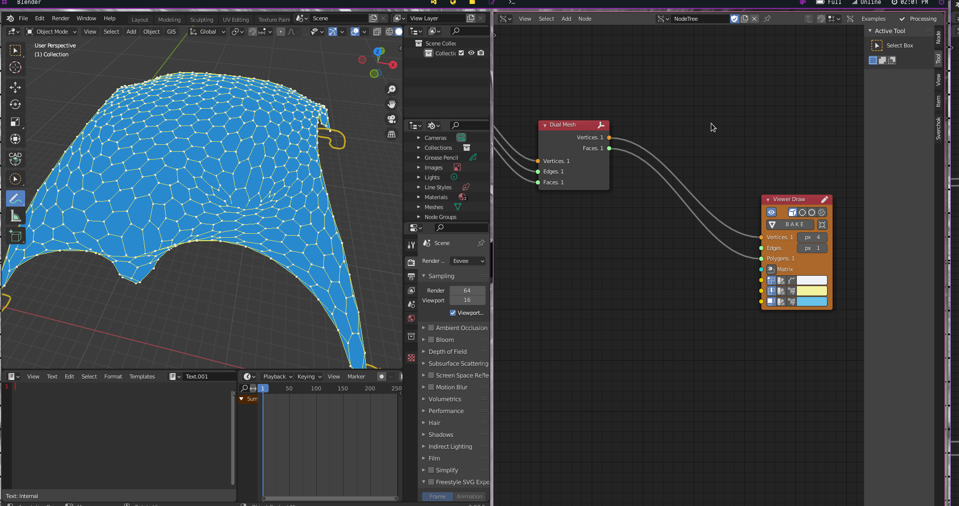
Then, we use the Dual Mesh(Modifiers -> Modifiers Make -> Dual Mesh) node to create the dual mesh based on the triangles. We connect the corresponding outputs from Triangulate Mesh into Dual Mesh input.
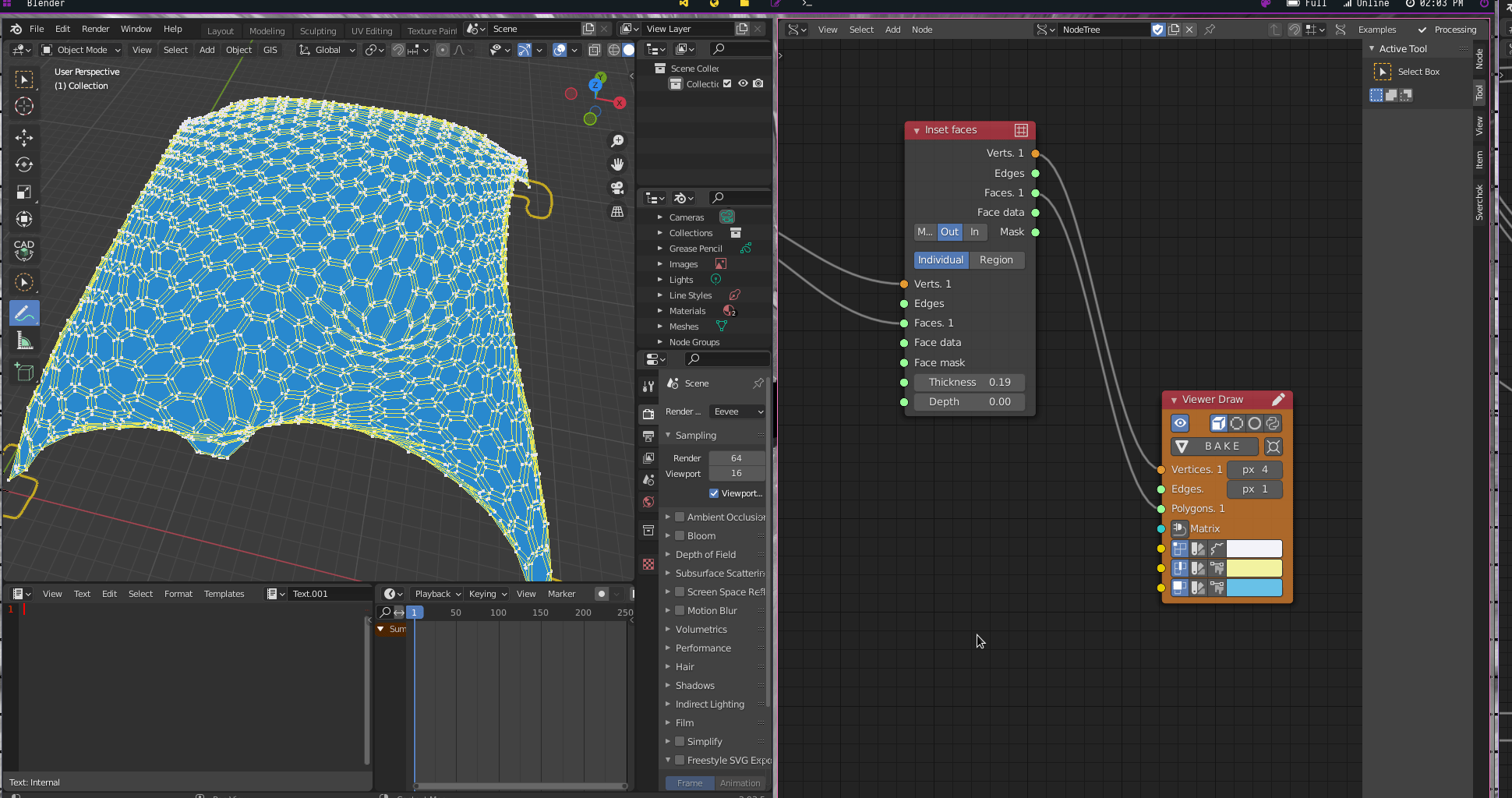
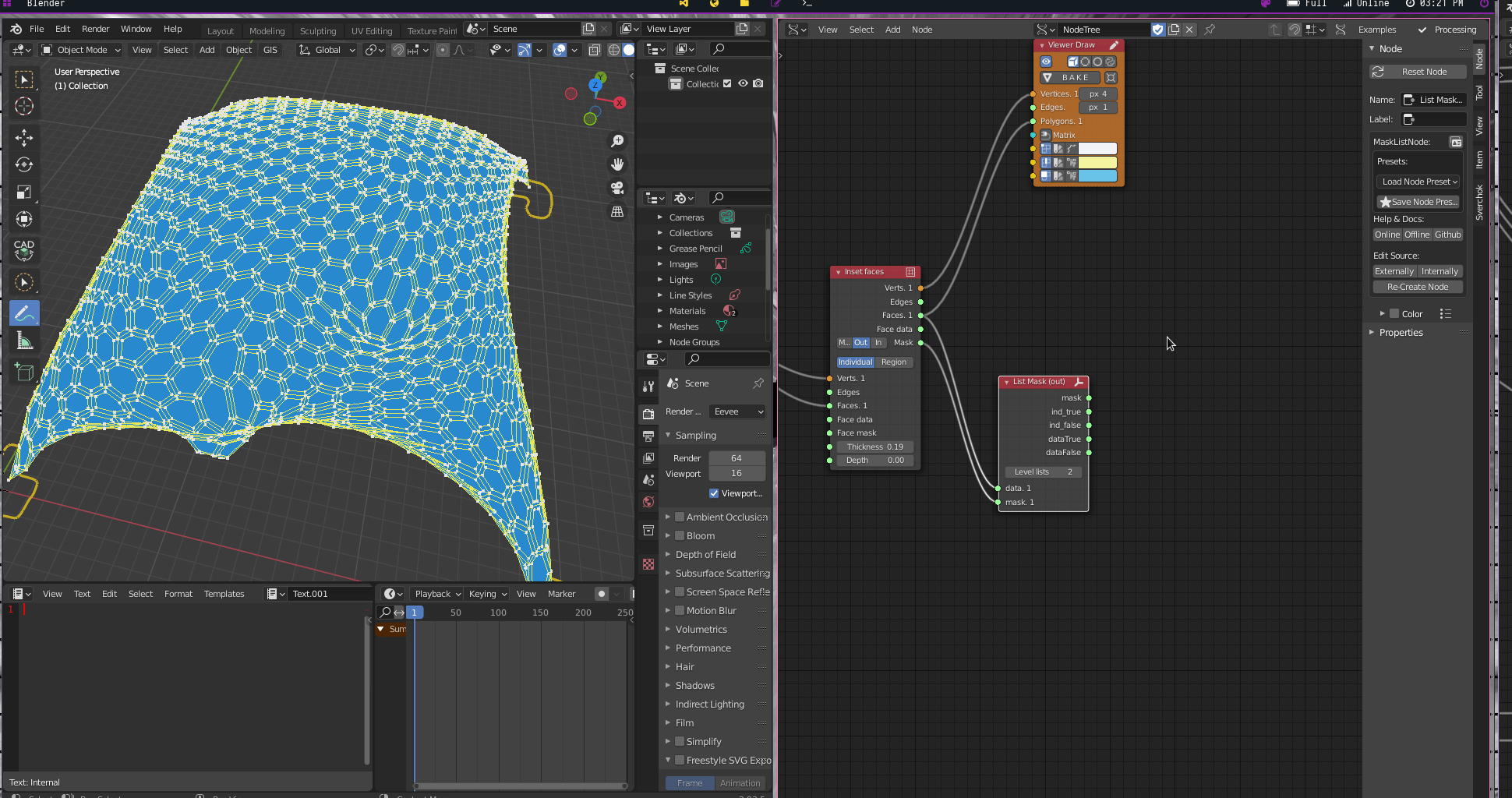
Now, we use Inset Faces(CAD -> Inset Faces) to create openings in the panels. We connect Dual Mesh output into Inset Faces input.
Inset Faces {Out; Individual; Thickness: 0.19}
Finally, we use a List Mask (Out)(List -> List Mask (Out)) node to filter opening and frames.
List Mask (Out) {Levels: 2}
Operations
Inset Faces [Faces ->]) -> ( List Mask (Out) [data <-])
Inset Faces [Mask ->]) -> ( List Mask (Out) [mask <-])
To finalise, we connect List Mask (Out) outputs in two Mesh Viewer(Viz -> Mesh Viewer) nodes.
Operations
(Inset Faces [Verts ->]) -> (Mesh Viewer [vertices <-])
(Inset Faces [Verts ->]) -> (Mesh Viewer (1) [vertices <-])
(List Mask (Out) [dataTrue ->]) -> (Mesh Viewer [Faces <-])
(List Mask (Out) [dataFalse ->]) -> (Mesh Viewer (1) [Faces <-])
Now, we can test change the random structural supports, trying to find a more appealing form.
You can download the blend file here
Have fun.