Waffle Struture
This is the last tutorial of the series, and I would like to close it with a script that is one of the most classical scripts in Grasshopper, the “Waffle Structure”. Also, it was one of the scripts that I first that I learnt in Grasshopper.
The “Waffle Structure” is a script that explores a key concept in Computational Design, the Digital Continuum (Kolarevic 2004). Kolarevic describes the process of File-to-Factory as a continuum through Design, Fabrication, and Assembly, using the same digital information during the whole process. The “Waffle Structure” is a good and simple example of this process in a small scale. For instance, we can cut the “Waffle Structure” using Laser Cutter and cardboard pieces to assemble the model. It is a fun exercise.
Let’s do it.
Building the Pavilion.
First, we create a shape for the pavilion. To keep it simple, we will focus on the creation of the structure. The idea is to use three arcs as a “barrel vault”.

We create the first arc using a Circle (Generator -> Circle) node. We change the variable Degrees to 180 to create a half-circle. Also, we use a Viewer Draw node to visualise it.
(Cirle [Vertices ->]) -> (Viewer Draw [ <- Vertices])
(Cirle [Edges ->]) -> (Viewer Draw [ <- Edges])
(Cirle [Polygons ->]) -> (Viewer Draw [ <- Polygons])

Then, we create a Number Range node with start=0, step=3, and count=3, connecting a Vector In into the variable Y to create coordinates (as vertices) for the other two arcs.
Number Range {Float ; Step}
(Number Range [Range ->]) -> (Vector In [Y <-])

We use a Matrix In (Matrix -> Matrix In) node to create three half circles based on the previous half circle. Also, we use a List Input(List -> List Main -> List Input) node to define scale factors for the half circles, creating a list of 3 Float numbers, 1, 0.6, and 1.5 respectively.
List Input {List Length : 3 ; Float}
(Vector In [Vectors ->]) -> (Matrix In [Location <-])
(List Input [List ->]) -> (Matrix In [Scale <-])

We apply the changes made by the Matrix In using Matrix Apply(Matrix -> Matrix Apply).
(Cirle [Vertices ->]) -> (Matrix Apply [ <- Vertices])
(Cirle [Edges ->]) -> (Matrix Apply [ <- Edges])
(Cirle [Polygons ->]) -> (Matrix Apply [ <- Faces])
(Matrix In [Matrix ->]) -> (Matrix Apply [Matrices [<-])
(Matrix Apply [Vertices ->]) -> (Viewer Draw [ <- Vertices])
(Matrix Apply [Edges ->]) -> (Viewer Draw [ <- Edges])
(Matrix Apply [Polygons ->]) -> (Viewer Draw [ <- Polygons])

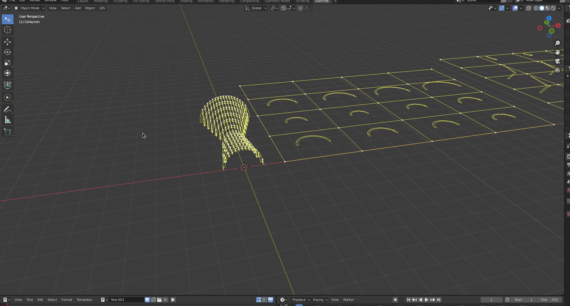
Then, we use a UV Connection(Modifiers -> Modifiers Change -> UV Connection) node to create barrel vault shape.
UV Connection {Direct: U ; Make : Pols}
(Matrix Apply [Vertices ->]) -> (UV Connection [ <- Vertices])
(UV Connection [Vertices ->]) -> (Viewer Draw [ <- Vertices])
(UV Connection [data ->]) -> (Viewer Draw [ <- Polygons])

We give some thickness to this shape using a Solidify(Modifiers -> Modifiers Make -> Solidify) node. We define the thickness variable as 0.1.
(UV Connection [Vertices ->]) -> (Solidify [ <- Vertices])
(UV Connection [data ->]) -> (Solidify [ <- Polygons])
(Solidify [Vertices ->]) -> (Viewer Draw (1) [ <- Vertices])
(Solidify [data ->]) -> (Viewer Draw (1) [ <- Polygons])

Now, we make a group with the pavilion Ctrl + j.

Creating Section Planes
To create the planes that will section the pavilion into beams, we first create planes in the X and Y directions. We start with a Number Range (1) node, defining start=0.27, step=0.52, and for count we can use an A Number(Number -> A Number) as an int=12.
Number Range (1) {Float; Step}
(A Number [->]) -> (Number Range (1) [count <-])

Then, we use a Vector In (1) node and a Matrix In (1) node to determine the planes’ location in Y direction.
(Number Range (1) [Range ->]) -> (Vector In (1)[Y <-])
(Vector In (1) [Vector ->]) -> (Matrix In (1)[Location <-])

Then, we create a List Repeater(List -> List Struct -> List Repeater) node to define angles for the planes. The right angle should be 90 degrees. However, when we create an intersection with 90, the fits will not be created properly. So, a trick that I use is to add 0.05 or 0.01, making sure that all the intersections will be created properly, it is not ideal, but it works for now. Also, we use a new A Number (1) to define the angle of 90.05. We use a Viewer Draw (2) node to visualise the planes.
List Repeater {level : 2 ; unwrap}
Matrix In {Angle : X : 1 ; Y : 0 ; Z : 0}
A Number (1) {float}
(A Number (1)[->]) -> (List Repeater [Data <-])
(List Repeater [Data ->]) -> (Matrix In (1) [Angle <-])

Now, we just copy and paste this block of nodes. We must change the copy of the Vector In (2)node fromYtoXto create the new planes onX`. We adjust the values to better intersect the shape with the new planes.


Then, we create a group for the planes Ctrl + j.

Creating Sections Beams
Now, we are ready to create the section beams. We create two Cross Section(CAD -> Cross Section) nodes, one for X and another for Y planes.
Cross Section {Fill Section; Alt+F/F}
Cross Section (1) {Fill Section; Alt+F/F}
(Solidify [Vertices ->]) -> (Cross Section [ <- Vertices])
(Solidify [data ->]) -> (Cross Section [ <- Polygons])
(Solidify [Vertices ->]) -> (Cross Section (1)[ <- Vertices])
(Solidify [data ->]) -> (Cross Section (1)[ <- Polygons])
(Matrix In (1) [Matrices ->]) -> (Cross Section [cut_matrix <-])
(Matrix In (2) [Matrices ->]) -> (Cross Section (1) [cut_matrix <-])
(Cross Section [Vertices ->]) -> (Viewer Draw (3) [Vertices <-])
(Cross Section [Edges ->]) -> (Viewer Draw (3) [Edges <-])
(Cross Section (1) [Vertices ->]) -> (Viewer Draw (4) [Vertices <-])
(Cross Section (1) [Edges ->]) -> (Viewer Draw (4) [Edges <-])

We have the section beams now, but we still need to create a section line that will guide the fits for the beams. To do that we create a new Cross Section node that intersects X beams with the Y planes.
(Cross Section [Vertices ->]) -> (Cross Section (2) [Vertices <-])
(Cross Section [Edges ->]) -> (Cross Section (2) [Edges <-])
(Matrix In (2) [Matrices ->]) -> (Cross Section (2) [cut_matrix <-])

Because we are dealing with mesh geometries, it is critical to control the precision of curves. For the intersection to work right, we must increase the number of subdivisions in the curved beam. To do that, we use two Subdivide Lite(Beta Nodes -> Subdivide Lite) nodes. The first one is for X beams (Cross Section), and another for Y beams (Cross Section (1)) with the cuts parameter equal to 10.
Subdivide Lite {Show Parameters ; cuts : 10 }
Subdivide Lite (1) {Show Parameters ; cuts : 10 }
(Cross Section [Vertices ->]) -> (Subdivide Lite [Vertices <-])
(Cross Section [Edges ->]) -> (Subdivide Lite [edg_pol <-])
(Cross Section (1) [Vertices ->]) -> (Subdivide Lite (1) [Vertices <-])
(Cross Section (1) [Edges ->]) -> (Subdivide Lite (1) [edg_pol <-])

The next step is to create fits. We use two Wafel(CAD -> Wafel) nodes to create the fits. Then, we use two Viewer Draw nodes to visualise the fits.
Wafel {UP; Threshold : 0 ; thick : 0.01}
Wafel (1) {DOWN; Threshold : 0 ; thick : 0.01}
(Cross Section (2) [Vertices ->]) -> (Wafel [vecLine <-])
(Cross Section (2) [Vertices ->]) -> (Wafel (1) [vecLine <-])
(Subdivide Lite [Vertices ->]) -> (Wafel [vecPlane <-])
(Subdivide Lite [Edges ->]) -> (Wafel [edgePlane <-])
(Subdivide Lite (1) [Vertices ->]) -> (Wafel (1) [vecPlane <-])
(Subdivide Lite (1) [Edges ->]) -> (Wafel (1) [edgePlane <-])
(Wafel [vert ->]) -> (Viewer Draw (4) [Vertices <-])
(Wafel [edge ->]) -> (Viewer Draw (4) [Edges <-])
(Wafel (1) [vert ->]) -> (Viewer Draw (5) [Vertices <-])
(Wafel (1) [edge ->]) -> (Viewer Draw (5) [Edges <-])
Then, we group the Waffle nodes Ctrl + j.

Orient the Waffle beams into XY axis.
The next step is to orient the beam into XY axis to be able to fabricate it later.
First, we create two Plane(Generator -> Plane) nodes to receive the beams. We adjust the values accordingly:
Plane {XY ; Num; NumX : 5 ; NumY : 5 ; StepX : 4.12 : StepY : 3.01}
Plane (1) {XY ; Num; NumX : 6 ; NumY : 6 ; StepX : 4.06 : StepY : 2.92}
Also, we use two Matrix In nodes to change the original starting point of the planes.
(Matrix In (3) [Matrices ->]) -> (Plane [Matrix <-])
(Matrix In (4) [Matrices ->]) -> (Plane (1)[Matrix <-])
(Plane [Vertices ->]) -> (Viewer Draw (6)[Vertices <-])
(Plane [Edges ->]) -> (Viewer Draw (6)[Edges <-])

We use two Origins(Analyzers-> Origins) to create centre points in the division of the plane. Then, we connect four Viewer Draw nodes to better visualise the planes and the centre vertices.
Origins {Faces}
Origins (1) {Faces}
(Plane [Vertices ->]) -> (Viewer Draw (7)[Vertices <-])
(Plane [Edges ->]) -> (Viewer Draw (7)[Edges <-])
(Plane [Vertices ->]) -> (Origins [Vertices <-])
(Plane [Edges ->]) -> (Origins [Edges <-])
(Plane [Polygons ->]) -> (Origins [Polygons <-])
(Plane (1) [Vertices ->]) -> (Viewer Draw (7)[Vertices <-])
(Plane (1) [Edges ->]) -> (Viewer Draw (7)[Edges <-])
(Plane (1) [Vertices ->]) -> (Origins (1) [Vertices <-])
(Plane (1) [Edges ->]) -> (Origins (1) [Edges <-])
(Plane (1) [Polygons ->]) -> (Origins (1) [Polygons <-])

Then, we use two List match nodes to get the shortest list between plane centre vertices and beams (it is critical that we have more centre vertices than beams). We connect the centre of Waffle beams and the Origins into the List Match nodes.
List Match {Level : 2 ; Short}
List Match (1) {Level : 2 ; Short}
(Wafel [centers ->]) -> (List Match [Data 0 <-])
(Origins [Origin ->]) -> (List Match [Data 1 <-])
(Wafel (1) [centers ->]) -> (List Match (1) [Data 0 <-])
(Origins (1) [Origin ->]) -> (List Match (1) [Data 1 <-])

Then, we use two Matrix In nodes two define the new location for the beams. We change the angle for -90 degrees.
(List Match [Data 1 ->]) -> (Matrix In (5) {Location <-])
(List Match (1) [Data 1 ->]) -> (Matrix In (6) {Location <-])

We use two Matrix Apply nodes to apply the changes.
(Wafel [vert ->]) -> (Matrix Apply (1) [Vertices <-])
(Wafel [edge ->]) -> (Matrix Apply (1) [Edges <-])
(Matrix In (5) [Matrices ->) -> (Matrix Apply (1) [Matrices <-)
(Wafel (1)[vert ->]) -> (Matrix Apply (2) [Vertices <-])
(Wafel (1) [edge ->]) -> (Matrix Apply (2) [Edges <-])
(Matrix In (6) [Matrices ->) -> (Matrix Apply (2) [Matrices <-)

We adjust the values for both last Matrix In nodes.
Matrix In (5){Axis : X : 1 ; Y: 0 ; Z : 0}
Matrix In (6){Axis : X : 1 ; Y: 1 ; Z : 0}
Then, we use two Vector Out and Vector In nodes to orient the beams in the XY, using the Z axis as 0.
(Matrix Apply [Vertices ->]) -> (Vector Out [vectors <-])
(Vector Out [X ->]) -> (Vector In (3)[X <-])
(Vector Out [Y ->]) -> (Vector In (3)[Y <-])
(Vector In (3) [Vectors ->]) -> (Viewer Draw (8) [Vertices <-])
(Matrix Apply (1) [Vertices ->]) -> (Vector Out (1) [vectors <-])
(Vector Out (1) [X ->]) -> (Vector In (4)[X <-])
(Vector Out (1) [Y ->]) -> (Vector In (4)[Y <-])
(Vector In (4) [Vectors ->]) -> (Viewer Draw (9) [Vertices <-])

Now we can create two groups for the beams, Ctrl +j.

Creating the SVG document
Now we can start to create a SVG file. We start defining the location for the beams labeling. We use two Text SVG(SVG -> text SVG) nodes, connecting List Match nodes.
Text SVG {start; normal; Text Size 0.2}
Text SVG (1) {start; normal; Text Size 0.2}
(List Match [Data 1 ->]) -> (Text SVG [Location <-)
(List Match (1) [Data 1 ->]) -> (Text SVG (1)[Location <-)
Then, we get the length of both List Match nodes using the List Length node.
(List Match [Data 1 ->]) -> (List Length (1) [Data <-)
(List Match (1) [Data 1 ->]) -> (List Length (2)[Data <-)

We create two Number Range nodes to enumerate the beams.
Number Range (2) {Int ; Step}
Number Range (3) {Int ; Step}
(List Length (1) [Length ->)-> (Number Range (2) [count <-])
(List Length (2) [Length ->)-> (Number Range (3)[count <-])

Then, we use two Formula(Script -> Formula) nodes to tag the beam.
The first one for X we define as :
str(x) + " U"
The second one for Y we define as:
str(x) + " Y"
(Number Range (2) [Range ->]) -> (Formula [x <-])
(Number Range (3) [Range ->]) -> (Formula [x <-])

Then, we connect corresponding texts into Text SVG nodes.

Next, we use two Mesh SVG(SVG -> Mesh SVG) nodes for the named beams U and V beams.
(Vector In (3) [Vectors ->]) -> (Mesh SVG [Vertices <-])
(Matrix Apply [Vertices ->]) -> (Mesh SVG [Polygons/Edges <-])
(Vector In (4) [Vectors ->]) -> (Mesh SVG (1) [Vertices <-])
(Matrix Apply (1) [Vertices ->]) -> (Mesh SVG (1) [Polygons/Edges <-])

We create a Fill/Stroke SVG(SVG -> Fill/Stroke) node to define a line thickness for the beams.
Fill/Stroke SVG {Blend ; Fill : None ; Stroke : Flat ; Stroke width : 0.01 }
(Fill/Stroke SVG [Fill/Stroke ->]) -> (Mesh SVG [Fill/Stroke <-])
(Fill/Stroke SVG [Fill/Stroke ->]) -> (Mesh SVG (1) [Fill/Stroke <-])

Then, we use a List Join(List -> List Main -> List Join) node to join all Mesh SVG and Text SVG lists.
(Mesh SVG [SVG Objects -> ]) -> (List Join [Data <-])
(Text SVG [SVG Objects -> ]) -> (List Join [Data 1 <-])
(Mesh SVG (1) [SVG Objects -> ]) -> (List Join [Data 2 <-])
(Text SVG (1) [SVG Objects -> ]) -> (List Join [Data 3 <-])

Finally, we use an SVG Document(`SVG -> SVG Document) node to define the SVG file. Also, we use a file path to save the SVG file.
SVG Document {Units : mm ; Width : 510 ; Height : 150 ; Scale : 10}
List Join [data ->]) -> (SVG Document [SVG Objects <-])
(File Path [File Path ->]) -> (SVG Document [Folder Path <-])

Then, we group the SVG nodes Ctrl + j.

Adjusting the Y planes to the barrel vault form (Bonus)
We made a classical Waffle structure with X and Y planes sectioning the shape. This strategy works well for several forms, but for this specific case, if we want to optimise the beam distribution in the Y axis, we might distribute the Y beams radially, following the curvature of the “barrel vault”.

To do that, we change the Y planes. We start creating a Circle (1) node using the same parameters as the original one that defines the shape. We create a new circle because we can control the number of divisions independently, changing the Num Verts parameter.
Circle (1) {Radius : 1 ; Degrees : 180 ; Num Verts : 11}

Then, we use a Matrix Apply (3) node using the same Matrix Deform that change the original Circle.
Circle (1) [Vertices ->]) -> (Matrix Apply (3) [Vertices <-])
Circle (1) [Edges ->]) -> (Matrix Apply (3) [Edges <-])
Circle (1) [Polygons ->]) -> (Matrix Apply (3) [Faces <-])
(Matrix Deform [Matrix ->]) -> (Matrix Apply (3) [Matrices <-])

Then, we use two List Item(List -> List Struct -> List Item) nodes to get the vertices and edges just from the first arc.
List Item {level : 1 ; index : 0}
List Item (1){level : 1 ; index : 0}
(Matrix Apply (3) [Vertices ->]) -> (List Item [data <-])
(Matrix Apply (3) [Edges ->]) -> (List Item (1)[data <-])

We use a Origins (1) node to create the planes from a matrix.
Origins (1) {Edges}
(List Item [Item ->]) -> (Origins [Verts <-])
(List Item (1) [Item ->]) -> (Origins [Edges <-])

Now, we create angles for the planes. We use List Length (2), A Number (2), and List Repeater (1). We get the number of vertices of the Circle (1) using List Length (2), then we define the angle with A Number (2) = 90.05 and List Repeater (1) to create a list of angles with the same length of the number of vertices of the Circle (1).
List Length (2) {level ; 1}
A Number (2) {float ; a float : 90.05}
List Repeater (1) {level : 2 ; unwrap}
Circle (1) [Vertices ->]) -> (List Length [Data <-])
A Number (2) [->]) -> (List Repeater (1) [Data <-])
List Length (2) [Length ->]) -> (List Repeater (1) [Number <-])

Then, we use a Matrix Deform (1) node to apply the changes into the planes. Also, we use a Vector In (4) with X=0, Y=1, Z=0 to define a rotation axis for the planes.
(Origins (1) [Matrix ->]) -> (Matrix Deform (1) [Original <-])
(Vector In (4) [Vectors ->]) -> (Matrix Deform (1) [Rotation <-])
(List Repeater (1) [Data ->]) -> (Matrix Deform (1) [Angle <-])

Then, we create a group with these planes Ctrl + j.

Finally, it the time to replace the Y planes with the new radial Y planes.
(Matrix Deform (1) [Matrix ->]) -> (Cross Section (1) [cut_matrix <-])
(Matrix Deform (1) [Matrix ->]) -> (Cross Section (2) [cut_matrix <-])

Now we have the Y beams distributed along the normal of the curve.
You can download the blend file here.
Have fun.

References
Kolarevic, B. ed., 2004. Architecture in the digital age: design and manufacturing. taylor & Francis.